import xgboost
import shap
import matplotlib.pyplot as plt
import numpy as np
import pandas as pd

# Import machine learning methods
from sklearn.model_selection import train_test_split
from xgboost import XGBClassifier
from lightgbm import LGBMClassifier
from sklearn.ensemble import RandomForestClassifier

# Import shap for shapley values
import shap

# JavaScript Important for the interactive charts later on
shap.initjs()15 SHAP with XGBoost (Titanic Dataset)
download_required = True

if download_required:

    # Download processed data:
    address = 'https://raw.githubusercontent.com/MichaelAllen1966/' + \
                '1804_python_healthcare/master/titanic/data/processed_data.csv'

    data = pd.read_csv(address)

    # Create a data subfolder if one does not already exist
    import os
    data_directory ='./datasets/'
    if not os.path.exists(data_directory):
        os.makedirs(data_directory)

    # Save data
    data.to_csv(data_directory + 'processed_data.csv', index=False)

data = pd.read_csv('datasets/processed_data.csv')
# Make all data 'float' type
data = data.astype(float)

# Use `survived` field as y, and drop for X
y = data['Survived'] # y = 'survived' column from 'data'
X = data.drop('Survived', axis=1) # X = all 'data' except the 'survived' column

# Drop PassengerId
X.drop('PassengerId',axis=1, inplace=True)

X_train, X_test, y_train, y_test = train_test_split(X,
                                                    y,
                                                    random_state=42,
                                                    test_size=0.25)

model = XGBClassifier(random_state=42)
model.fit(X_train, y_train)

# Predict training and test set labels
y_pred_train = model.predict(X_train)
y_pred_test = model.predict(X_test)

# Predict probabilities of survival
y_prob_train = model.predict_proba(X_train)
y_prob_test = model.predict_proba(X_test)

accuracy_train = np.mean(y_pred_train == y_train)
accuracy_test = np.mean(y_pred_test == y_test)

print (f'Accuracy of predicting training data = {accuracy_train:.2%}')
print (f'Accuracy of predicting test data = {accuracy_test:.2%}')
Accuracy of predicting training data = 97.31%
Accuracy of predicting test data = 80.72%# explain the model's predictions using SHAP
explainer = shap.Explainer(model, X_train)
shap_values = explainer(X_test)
shap_values.values =
array([[-0.41472028, -0.82758431,  0.08631781, ...,  0.        ,
         0.        ,  0.        ],
       [ 0.34368675,  0.01027041,  0.20749824, ...,  0.        ,
         0.        ,  0.        ],
       [-0.49629094, -0.24858944, -0.07239207, ...,  0.        ,
         0.        ,  0.        ],
       ...,
       [-0.45505765, -0.95988004,  0.14636154, ...,  0.        ,
         0.        ,  0.        ],
       [ 1.38846514, -0.87314281,  0.06420199, ...,  0.        ,
         0.        ,  0.        ],
       [-0.51810456, -1.0059387 ,  0.18350499, ...,  0.        ,
         0.        ,  0.        ]])
.base_values =
array([-0.81725838, -0.81725838, -0.81725838, -0.81725838, -0.81725838,
-0.81725838, -0.81725838, -0.81725838, -0.81725838, -0.81725838,
-0.81725838, -0.81725838, -0.81725838, -0.81725838, -0.81725838,
-0.81725838, -0.81725838, -0.81725838, -0.81725838, -0.81725838,
-0.81725838, -0.81725838, -0.81725838, -0.81725838, -0.81725838,
-0.81725838, -0.81725838, -0.81725838, -0.81725838, -0.81725838,
-0.81725838, -0.81725838, -0.81725838, -0.81725838, -0.81725838,
-0.81725838, -0.81725838, -0.81725838, -0.81725838, -0.81725838,
-0.81725838, -0.81725838, -0.81725838, -0.81725838, -0.81725838,
-0.81725838, -0.81725838, -0.81725838, -0.81725838, -0.81725838,
-0.81725838, -0.81725838, -0.81725838, -0.81725838, -0.81725838,
-0.81725838, -0.81725838, -0.81725838, -0.81725838, -0.81725838,
-0.81725838, -0.81725838, -0.81725838, -0.81725838, -0.81725838,
-0.81725838, -0.81725838, -0.81725838, -0.81725838, -0.81725838,
-0.81725838, -0.81725838, -0.81725838, -0.81725838, -0.81725838,
-0.81725838, -0.81725838, -0.81725838, -0.81725838, -0.81725838,
-0.81725838, -0.81725838, -0.81725838, -0.81725838, -0.81725838,
-0.81725838, -0.81725838, -0.81725838, -0.81725838, -0.81725838,
-0.81725838, -0.81725838, -0.81725838, -0.81725838, -0.81725838,
-0.81725838, -0.81725838, -0.81725838, -0.81725838, -0.81725838,
-0.81725838, -0.81725838, -0.81725838, -0.81725838, -0.81725838,
-0.81725838, -0.81725838, -0.81725838, -0.81725838, -0.81725838,
-0.81725838, -0.81725838, -0.81725838, -0.81725838, -0.81725838,
-0.81725838, -0.81725838, -0.81725838, -0.81725838, -0.81725838,
-0.81725838, -0.81725838, -0.81725838, -0.81725838, -0.81725838,
-0.81725838, -0.81725838, -0.81725838, -0.81725838, -0.81725838,
-0.81725838, -0.81725838, -0.81725838, -0.81725838, -0.81725838,
-0.81725838, -0.81725838, -0.81725838, -0.81725838, -0.81725838,
-0.81725838, -0.81725838, -0.81725838, -0.81725838, -0.81725838,
-0.81725838, -0.81725838, -0.81725838, -0.81725838, -0.81725838,
-0.81725838, -0.81725838, -0.81725838, -0.81725838, -0.81725838,
-0.81725838, -0.81725838, -0.81725838, -0.81725838, -0.81725838,
-0.81725838, -0.81725838, -0.81725838, -0.81725838, -0.81725838,
-0.81725838, -0.81725838, -0.81725838, -0.81725838, -0.81725838,
-0.81725838, -0.81725838, -0.81725838, -0.81725838, -0.81725838,
-0.81725838, -0.81725838, -0.81725838, -0.81725838, -0.81725838,
-0.81725838, -0.81725838, -0.81725838, -0.81725838, -0.81725838,
-0.81725838, -0.81725838, -0.81725838, -0.81725838, -0.81725838,
-0.81725838, -0.81725838, -0.81725838, -0.81725838, -0.81725838,
-0.81725838, -0.81725838, -0.81725838, -0.81725838, -0.81725838,
-0.81725838, -0.81725838, -0.81725838, -0.81725838, -0.81725838,
-0.81725838, -0.81725838, -0.81725838, -0.81725838, -0.81725838,
-0.81725838, -0.81725838, -0.81725838, -0.81725838, -0.81725838,
-0.81725838, -0.81725838, -0.81725838, -0.81725838, -0.81725838,
-0.81725838, -0.81725838, -0.81725838])
.data =
array([[ 3., 28., 1., ..., 0., 0., 1.],
[ 2., 31., 0., ..., 0., 0., 1.],
[ 3., 20., 0., ..., 0., 0., 1.],
...,
[ 3., 28., 0., ..., 0., 0., 1.],
[ 2., 24., 0., ..., 0., 0., 1.],
[ 3., 18., 1., ..., 0., 0., 1.]])shap_values_numeric = shap_values.values
shap_values_numericarray([[-0.41472028, -0.82758431, 0.08631781, ..., 0. ,
0. , 0. ],
[ 0.34368675, 0.01027041, 0.20749824, ..., 0. ,
0. , 0. ],
[-0.49629094, -0.24858944, -0.07239207, ..., 0. ,
0. , 0. ],
...,
[-0.45505765, -0.95988004, 0.14636154, ..., 0. ,
0. , 0. ],
[ 1.38846514, -0.87314281, 0.06420199, ..., 0. ,
0. , 0. ],
[-0.51810456, -1.0059387 , 0.18350499, ..., 0. ,
0. , 0. ]])16 SHAP - importance table
# Calculate mean Shap value for each feature in training set
importances = pd.DataFrame()
importances['features'] = X.columns.tolist()
importances['mean_shap_values'] = np.mean(shap_values_numeric, axis=0)

# Calculate mean absolute Shap value for each feature in training set
# This will give us the average importance of each feature
importances['mean_abs_shap_values'] = np.mean(
    np.abs(shap_values_numeric),axis=0)

importances['rank_shap'] = importances['mean_abs_shap_values'].rank(ascending=False).values
importances.sort_values('rank_shap').head()| features | mean_shap_values | mean_abs_shap_values | rank_shap | |
|---|---|---|---|---|
| 10 | male | 0.047098 | 1.872651 | 1.0 |
| 0 | Pclass | 0.268006 | 1.072309 | 2.0 |
| 4 | Fare | 0.084978 | 0.914949 | 3.0 |
| 1 | Age | -0.325160 | 0.846433 | 4.0 |
| 8 | CabinNumber | 0.126974 | 0.344576 | 5.0 |
17 SHAP Plots
shap.plots.bar(shap_values)
# visualize the first prediction's explanation
shap.plots.waterfall(shap_values[0])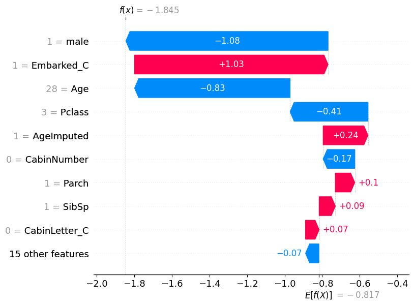
X_test[['male', 'Embarked_C', 'Age', 'Pclass']]| male | Embarked_C | Age | Pclass | |
|---|---|---|---|---|
| 709 | 1.0 | 1.0 | 28.0 | 3.0 |
| 439 | 1.0 | 0.0 | 31.0 | 2.0 |
| 840 | 1.0 | 0.0 | 20.0 | 3.0 |
| 720 | 0.0 | 0.0 | 6.0 | 2.0 |
| 39 | 0.0 | 1.0 | 14.0 | 3.0 |
| ... | ... | ... | ... | ... |
| 880 | 0.0 | 0.0 | 25.0 | 2.0 |
| 425 | 1.0 | 0.0 | 28.0 | 3.0 |
| 101 | 1.0 | 0.0 | 28.0 | 3.0 |
| 199 | 0.0 | 0.0 | 24.0 | 2.0 |
| 424 | 1.0 | 0.0 | 18.0 | 3.0 |
223 rows × 4 columns
# visualize another prediction's explanation
shap.plots.waterfall(shap_values[7])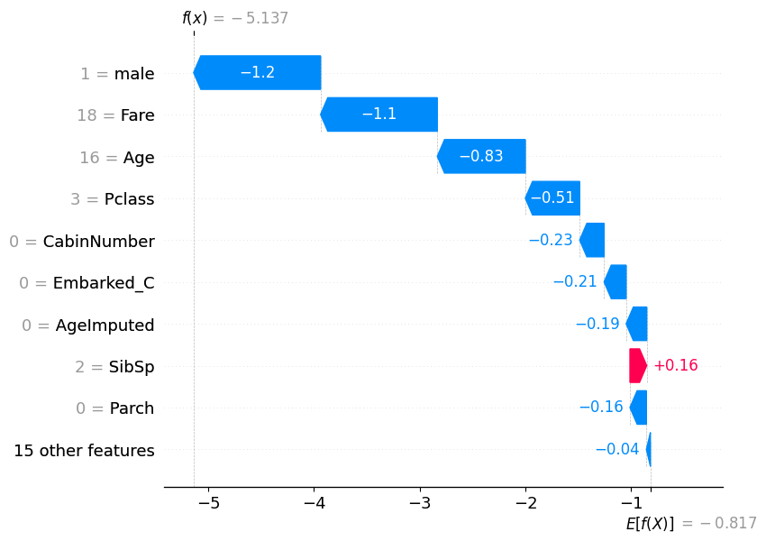
17.0.0.1 Find examples with high or low probabilities
highest_prob = pd.Series(y_pred_test).sort_values(ascending=False).head(1)
highest_prob
69 1
dtype: int32high_prob_index = highest_prob.index[0]
shap.plots.waterfall(shap_values[high_prob_index])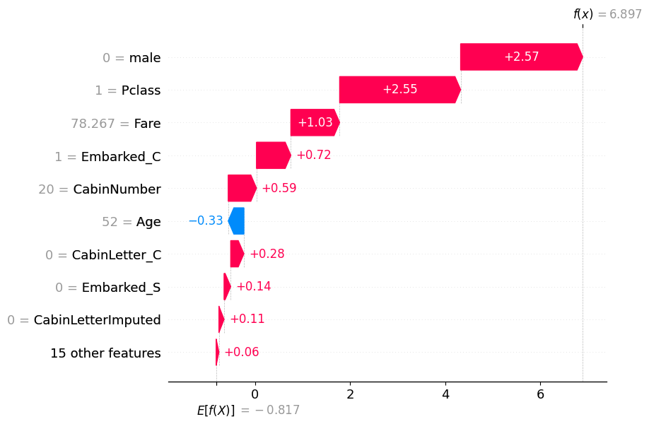
low_prob = pd.Series(y_pred_test).sort_values(ascending=False).tail(1)
low_prob
222 0
dtype: int32low_prob_index = low_prob.index[0]
shap.plots.waterfall(shap_values[low_prob_index])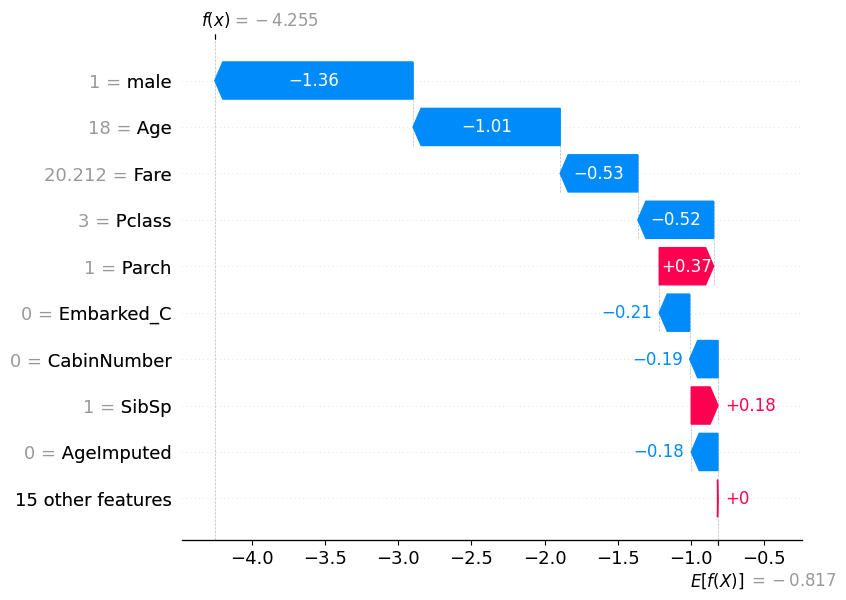
17.1 Force plots
# visualize the first prediction's explanation with a force plot
shap.plots.force(shap_values[0])
Visualization omitted, Javascript library not loaded!
Have you run `initjs()` in this notebook? If this notebook was from another user you must also trust this notebook (File -> Trust notebook). If you are viewing this notebook on github the Javascript has been stripped for security. If you are using JupyterLab this error is because a JupyterLab extension has not yet been written.
Have you run `initjs()` in this notebook? If this notebook was from another user you must also trust this notebook (File -> Trust notebook). If you are viewing this notebook on github the Javascript has been stripped for security. If you are using JupyterLab this error is because a JupyterLab extension has not yet been written.
# visualize all the predictions
shap.plots.force(shap_values)
Visualization omitted, Javascript library not loaded!
Have you run `initjs()` in this notebook? If this notebook was from another user you must also trust this notebook (File -> Trust notebook). If you are viewing this notebook on github the Javascript has been stripped for security. If you are using JupyterLab this error is because a JupyterLab extension has not yet been written.
Have you run `initjs()` in this notebook? If this notebook was from another user you must also trust this notebook (File -> Trust notebook). If you are viewing this notebook on github the Javascript has been stripped for security. If you are using JupyterLab this error is because a JupyterLab extension has not yet been written.
17.2 Dependence Plots
# create a dependence scatter plot to show the effect of a single feature across the whole dataset
shap.plots.scatter(shap_values[:, "Age"])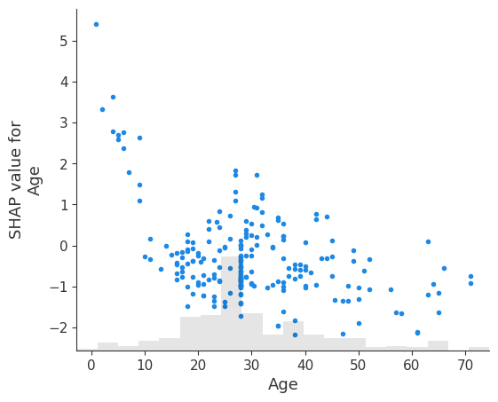
shap.plots.scatter(shap_values[:, "Age"], color=shap_values[:, "male"])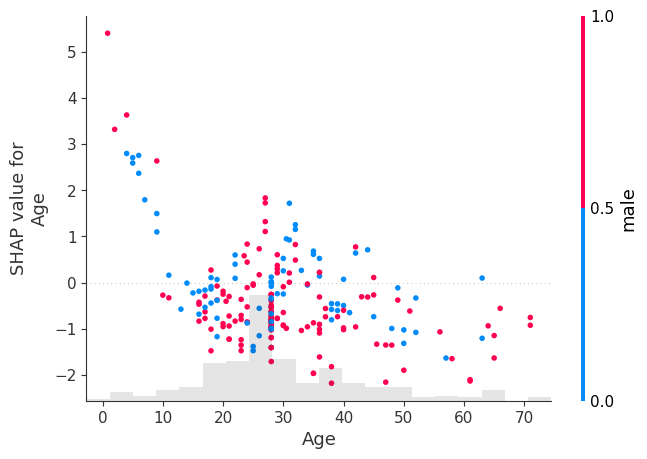
shap.plots.scatter(shap_values[:, "Age"], color=shap_values[:, "Pclass"])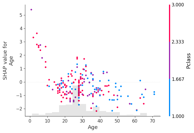
shap.plots.scatter(shap_values[:, "Age"], color=shap_values[:, "Fare"])
shap.plots.scatter(shap_values[:, "Age"], color=shap_values)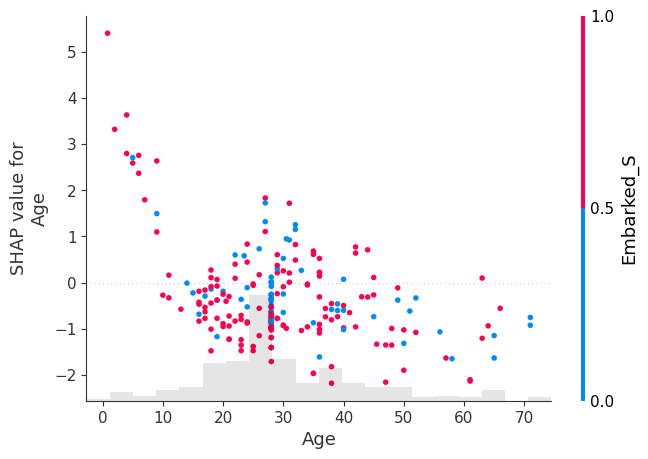
shap.plots.scatter(shap_values[:, "Fare"], color=shap_values)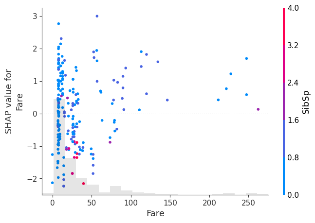
shap.plots.scatter(shap_values[:, "male"], color=shap_values)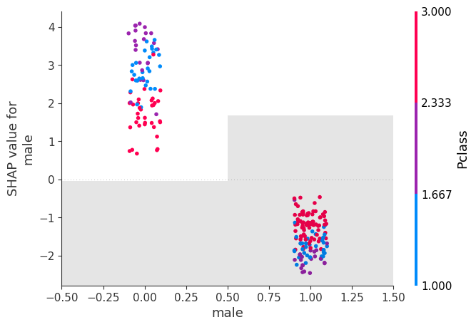
shap.plots.scatter(shap_values[:, "male"], color=shap_values)17.3 Beeswarm
# summarize the effects of all the features
shap.plots.beeswarm(shap_values)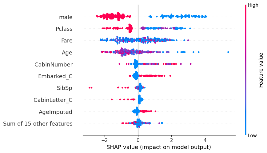
17.4 Violin
# summarize the effects of all the features
shap.plots.violin(shap_values)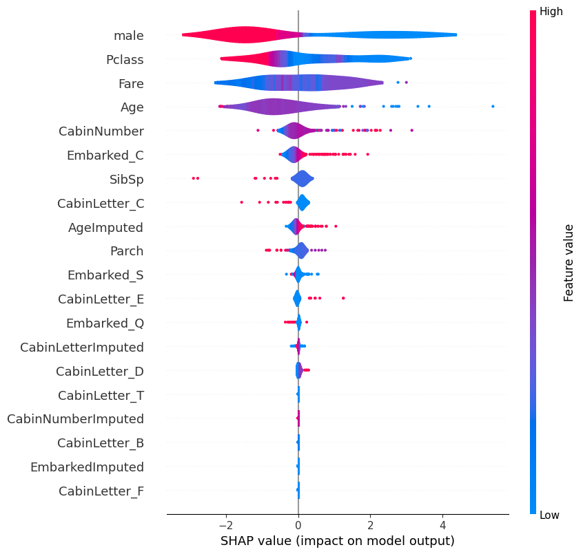
17.4.1 Bar: Cohorts
sex = ["Women" if shap_values[i, "male"].data == 0 else "Men" for i in range(shap_values.shape[0])]
shap.plots.bar(shap_values.cohorts(sex).abs.mean(0))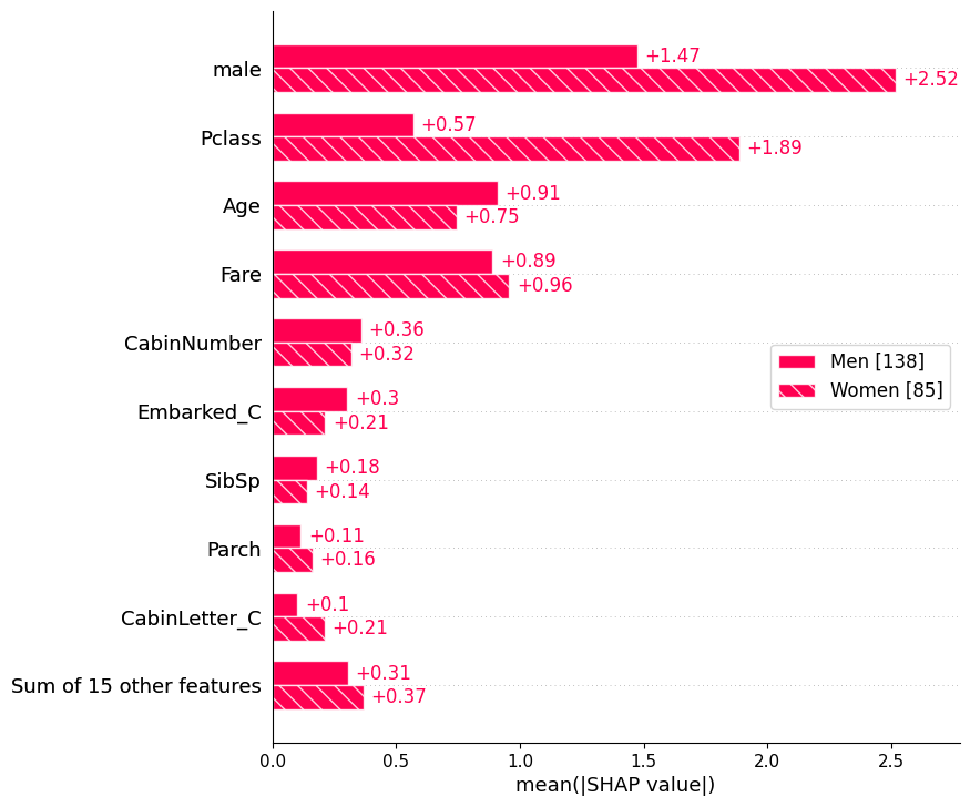
Plot the bars for an individual.
shap.plots.bar(shap_values[1])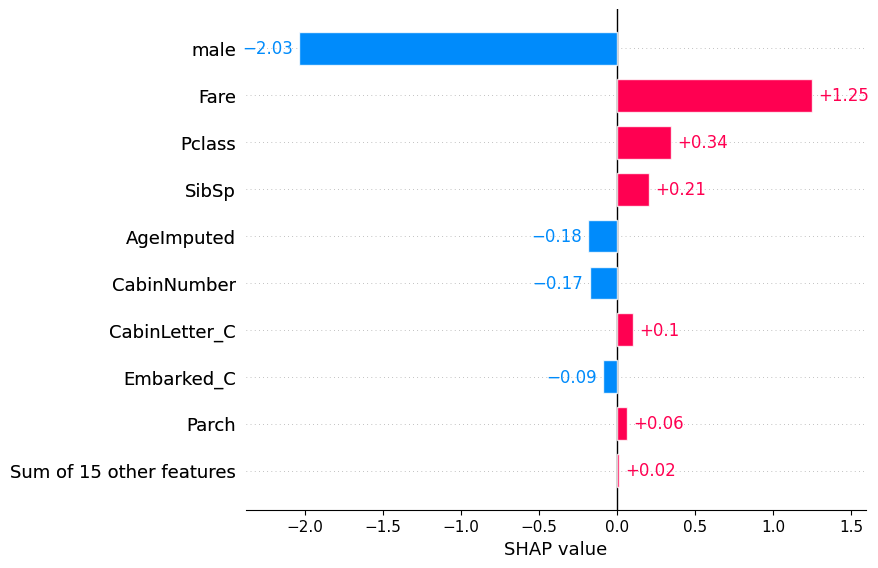
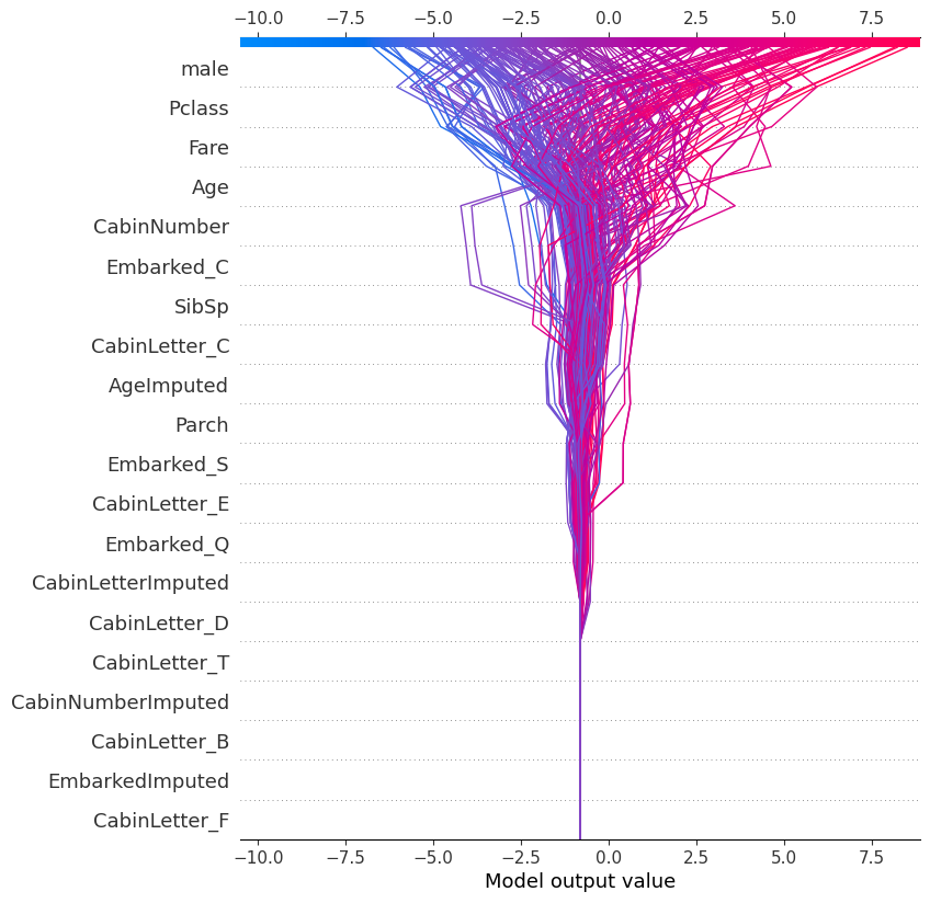
18 Decision
shap.plots.decision(
    explainer.expected_value,
    shap_values.values,
    feature_names=X.columns.tolist()
    )
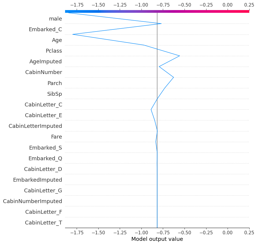
18.0.1 Decision plot for individual
shap.plots.decision(
    explainer.expected_value,
    explainer.shap_values(X_test)[0], # one way of specifying the record to look at
    feature_names=X.columns.tolist()
    )
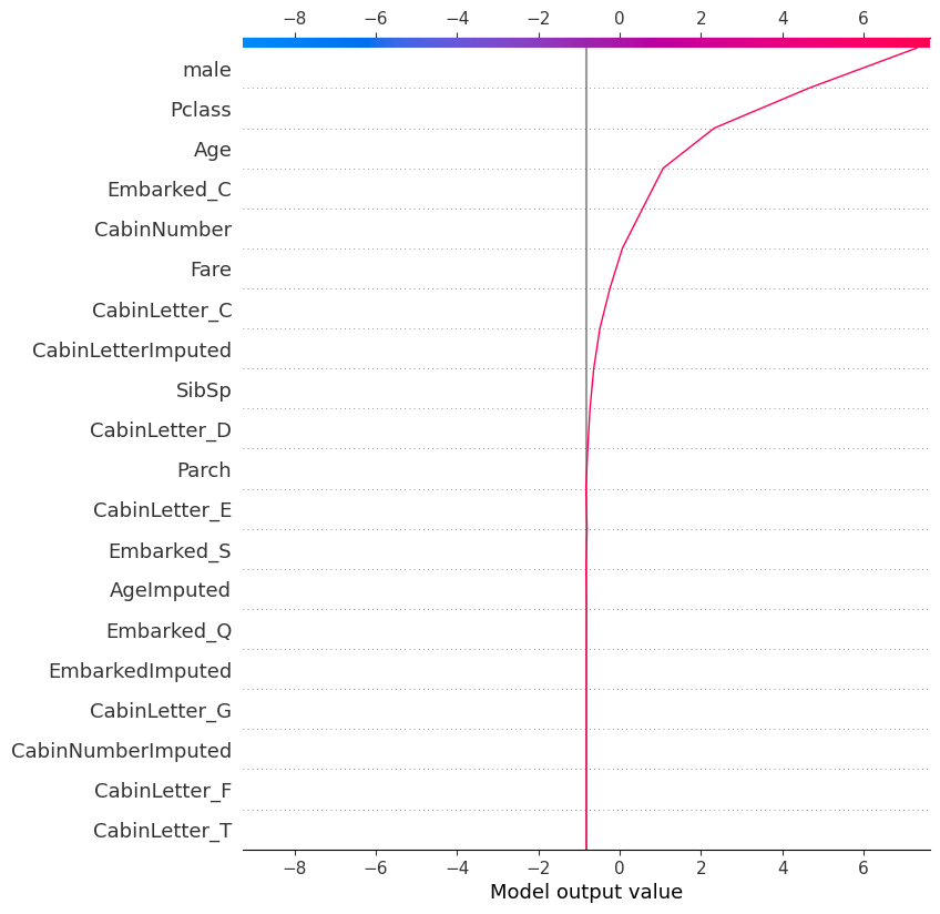
shap.plots.decision(
    explainer.expected_value,
    shap_values.values[121], # another way of specifying the record to look at
    feature_names=X.columns.tolist()
    )
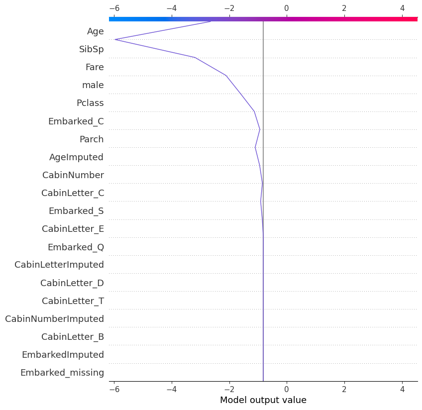
shap.plots.decision(
    explainer.expected_value,
    explainer.shap_values(X_test)[215],
    feature_names=X.columns.tolist()
    )
18.1 SHAP: Probability Alternative
Recalculate the SHAP values as changes in probability instead of log odds.
# explain the model's predictions using SHAP
explainer_probability = shap.Explainer(model, X_train, model_output="probability")
shap_values_probability = explainer_probability(X_test)

shap_values_probability
.values =
array([[-0.05238777, -0.13358663, 0.01009056, ..., 0. ,
0. , 0. ],
[ 0.0511844 , -0.03143588, 0.0286387 , ..., 0. ,
0. , 0. ],
[-0.05579166, -0.05355721, -0.00460973, ..., 0. ,
0. , 0. ],
...,
[-0.0458467 , -0.10278892, 0.01064102, ..., 0. ,
0. , 0. ],
[ 0.14912559, -0.06840275, 0.00767626, ..., 0. ,
0. , 0. ],
[-0.04991312, -0.10697621, 0.00952425, ..., 0. ,
0. , 0. ]])
.base_values =
array([0.38372332, 0.38372332, 0.38372332, 0.38372332, 0.38372332,
0.38372332, 0.38372332, 0.38372332, 0.38372332, 0.38372332,
0.38372332, 0.38372332, 0.38372332, 0.38372332, 0.38372332,
0.38372332, 0.38372332, 0.38372332, 0.38372332, 0.38372332,
0.38372332, 0.38372332, 0.38372332, 0.38372332, 0.38372332,
0.38372332, 0.38372332, 0.38372332, 0.38372332, 0.38372332,
0.38372332, 0.38372332, 0.38372332, 0.38372332, 0.38372332,
0.38372332, 0.38372332, 0.38372332, 0.38372332, 0.38372332,
0.38372332, 0.38372332, 0.38372332, 0.38372332, 0.38372332,
0.38372332, 0.38372332, 0.38372332, 0.38372332, 0.38372332,
0.38372332, 0.38372332, 0.38372332, 0.38372332, 0.38372332,
0.38372332, 0.38372332, 0.38372332, 0.38372332, 0.38372332,
0.38372332, 0.38372332, 0.38372332, 0.38372332, 0.38372332,
0.38372332, 0.38372332, 0.38372332, 0.38372332, 0.38372332,
0.38372332, 0.38372332, 0.38372332, 0.38372332, 0.38372332,
0.38372332, 0.38372332, 0.38372332, 0.38372332, 0.38372332,
0.38372332, 0.38372332, 0.38372332, 0.38372332, 0.38372332,
0.38372332, 0.38372332, 0.38372332, 0.38372332, 0.38372332,
0.38372332, 0.38372332, 0.38372332, 0.38372332, 0.38372332,
0.38372332, 0.38372332, 0.38372332, 0.38372332, 0.38372332,
0.38372332, 0.38372332, 0.38372332, 0.38372332, 0.38372332,
0.38372332, 0.38372332, 0.38372332, 0.38372332, 0.38372332,
0.38372332, 0.38372332, 0.38372332, 0.38372332, 0.38372332,
0.38372332, 0.38372332, 0.38372332, 0.38372332, 0.38372332,
0.38372332, 0.38372332, 0.38372332, 0.38372332, 0.38372332,
0.38372332, 0.38372332, 0.38372332, 0.38372332, 0.38372332,
0.38372332, 0.38372332, 0.38372332, 0.38372332, 0.38372332,
0.38372332, 0.38372332, 0.38372332, 0.38372332, 0.38372332,
0.38372332, 0.38372332, 0.38372332, 0.38372332, 0.38372332,
0.38372332, 0.38372332, 0.38372332, 0.38372332, 0.38372332,
0.38372332, 0.38372332, 0.38372332, 0.38372332, 0.38372332,
0.38372332, 0.38372332, 0.38372332, 0.38372332, 0.38372332,
0.38372332, 0.38372332, 0.38372332, 0.38372332, 0.38372332,
0.38372332, 0.38372332, 0.38372332, 0.38372332, 0.38372332,
0.38372332, 0.38372332, 0.38372332, 0.38372332, 0.38372332,
0.38372332, 0.38372332, 0.38372332, 0.38372332, 0.38372332,
0.38372332, 0.38372332, 0.38372332, 0.38372332, 0.38372332,
0.38372332, 0.38372332, 0.38372332, 0.38372332, 0.38372332,
0.38372332, 0.38372332, 0.38372332, 0.38372332, 0.38372332,
0.38372332, 0.38372332, 0.38372332, 0.38372332, 0.38372332,
0.38372332, 0.38372332, 0.38372332, 0.38372332, 0.38372332,
0.38372332, 0.38372332, 0.38372332, 0.38372332, 0.38372332,
0.38372332, 0.38372332, 0.38372332, 0.38372332, 0.38372332,
0.38372332, 0.38372332, 0.38372332, 0.38372332, 0.38372332,
0.38372332, 0.38372332, 0.38372332])
.data =
array([[ 3., 28., 1., ..., 0., 0., 1.],
[ 2., 31., 0., ..., 0., 0., 1.],
[ 3., 20., 0., ..., 0., 0., 1.],
...,
[ 3., 28., 0., ..., 0., 0., 1.],
[ 2., 24., 0., ..., 0., 0., 1.],
[ 3., 18., 1., ..., 0., 0., 1.]])18.1.1 Beeswarm Plot: Probability
shap.plots.beeswarm(shap_values_probability)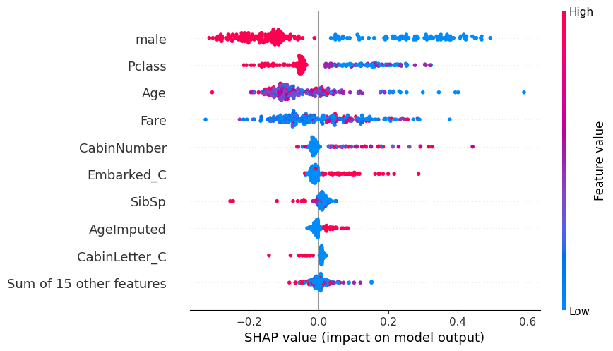
18.1.1.1 Comparison with log odds plot
fig, (ax1, ax2) = plt.subplots(nrows=2, ncols=1, figsize=(10,20))

plt.sca(ax1) ## NEW
shap.plots.beeswarm(shap_values, show=False)
plt.title("Log Odds")

# Change to the second axis
plt.sca(ax2) ## NEW
shap.plots.beeswarm(shap_values_probability, show=False)
plt.title("Probability")
plt.tight_layout()
plt.show()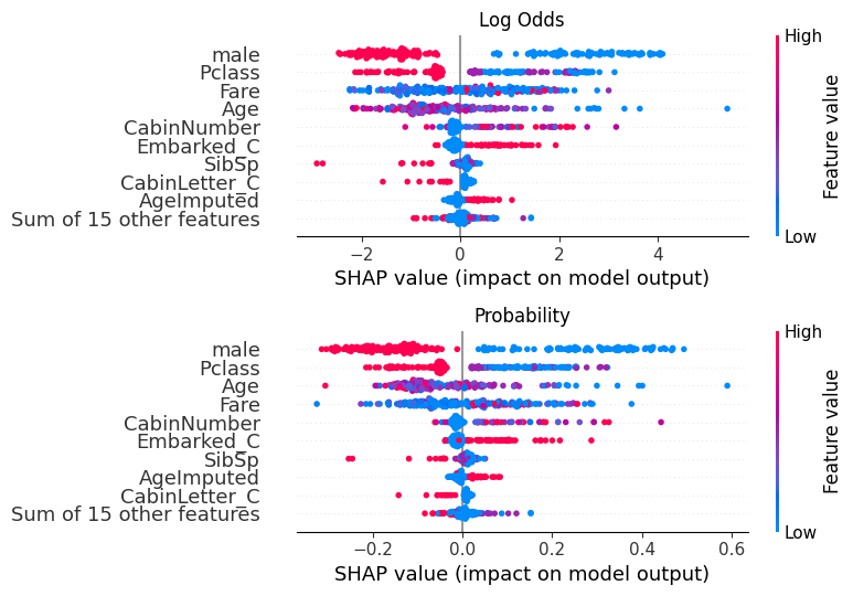
18.1.2 Waterfall Plot: Probability
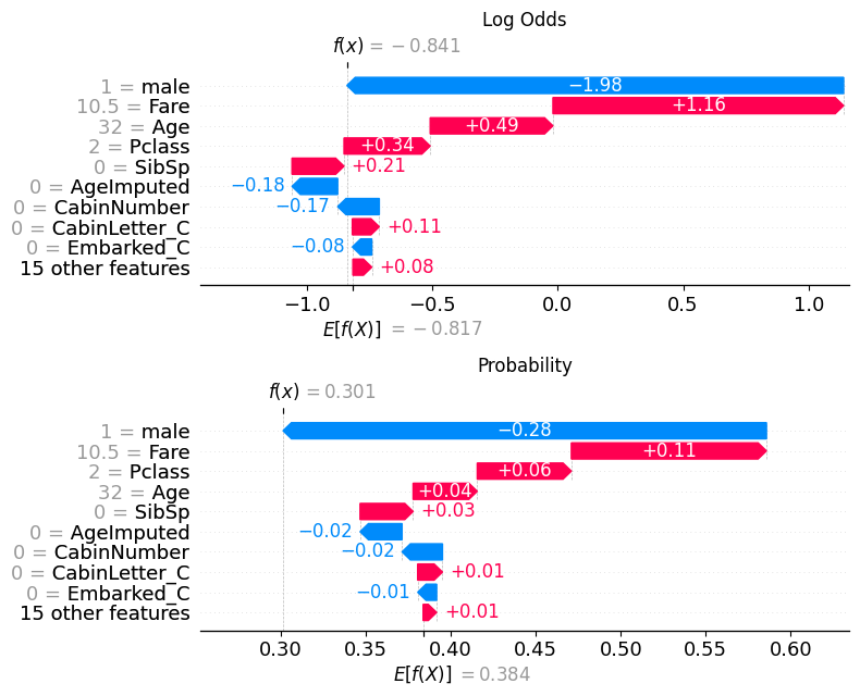
If we pull out the predicted probability for this passenger, we can see that the predicted probability of class 0 (died) is 0.69, while the predicted probability of survival (class 1) is 0.301.
pd.DataFrame(model.predict_proba(X_test)).reset_index(drop=True).iloc[56]0 0.69867
1 0.30133
Name: 56, dtype: float32This matches what is now shown in the waterfall plot.
shap.plots.waterfall(shap_values_probability[56])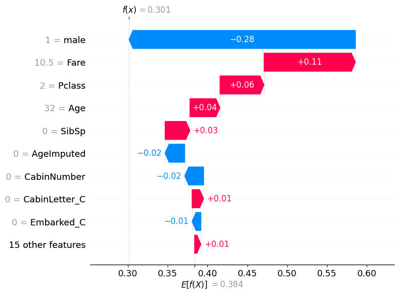
pd.DataFrame(model.predict_proba(X_test)).reset_index(drop=True).iloc[115]0 0.97308
1 0.02692
Name: 115, dtype: float32shap.plots.waterfall(shap_values_probability[115])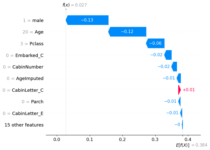
pd.DataFrame(model.predict_proba(X_test)).reset_index(drop=True).iloc[195]0 0.000583
1 0.999417
Name: 195, dtype: float32shap.plots.waterfall(shap_values_probability[195])
18.1.2.1 Comparison with log odds plot
fig, (ax1, ax2) = plt.subplots(nrows=2, ncols=1, figsize=(10,20))

plt.sca(ax1) ## NEW
shap.plots.waterfall(shap_values[56], show=False)
plt.title("Log Odds")
# Change to the second axis
plt.sca(ax2) ## NEW
shap.plots.waterfall(shap_values_probability[56], show=False)
plt.title("Probability")
plt.tight_layout()
plt.show()