6  Random Forests for Classification (Titanic Dataset)

import numpy as np
import pandas as pd
# Import machine learning methods
from sklearn.ensemble import RandomForestClassifier
from sklearn.model_selection import train_test_split
from sklearn.tree import plot_tree

import plotly.express as px
import matplotlib.pyplot as plt
%matplotlib inline


from sklearn.metrics import auc, roc_curve, RocCurveDisplay, f1_score, precision_score, \
                            recall_score, confusion_matrix, ConfusionMatrixDisplay

download_required = True

if download_required:

    # Download processed data:
    address = 'https://raw.githubusercontent.com/MichaelAllen1966/' + \
                '1804_python_healthcare/master/titanic/data/processed_data.csv'

    data = pd.read_csv(address)

    # Create a data subfolder if one does not already exist
    import os
    data_directory ='../datasets/'
    if not os.path.exists(data_directory):
        os.makedirs(data_directory)

    # Save data
    data.to_csv(data_directory + 'processed_titanic_data.csv', index=False)

data = pd.read_csv('../datasets/processed_titanic_data.csv')
# Make all data 'float' type
data = data.astype(float)

data.head(10)

	PassengerId	Survived	Pclass	Age	SibSp	Parch	Fare	AgeImputed	EmbarkedImputed	CabinLetterImputed	...	Embarked_missing	CabinLetter_A	CabinLetter_B	CabinLetter_C	CabinLetter_D	CabinLetter_E	CabinLetter_F	CabinLetter_G	CabinLetter_T	CabinLetter_missing
0	1.0	0.0	3.0	22.0	1.0	0.0	7.2500	0.0	0.0	1.0	...	0.0	0.0	0.0	0.0	0.0	0.0	0.0	0.0	0.0	1.0
1	2.0	1.0	1.0	38.0	1.0	0.0	71.2833	0.0	0.0	0.0	...	0.0	0.0	0.0	1.0	0.0	0.0	0.0	0.0	0.0	0.0
2	3.0	1.0	3.0	26.0	0.0	0.0	7.9250	0.0	0.0	1.0	...	0.0	0.0	0.0	0.0	0.0	0.0	0.0	0.0	0.0	1.0
3	4.0	1.0	1.0	35.0	1.0	0.0	53.1000	0.0	0.0	0.0	...	0.0	0.0	0.0	1.0	0.0	0.0	0.0	0.0	0.0	0.0
4	5.0	0.0	3.0	35.0	0.0	0.0	8.0500	0.0	0.0	1.0	...	0.0	0.0	0.0	0.0	0.0	0.0	0.0	0.0	0.0	1.0
5	6.0	0.0	3.0	28.0	0.0	0.0	8.4583	1.0	0.0	1.0	...	0.0	0.0	0.0	0.0	0.0	0.0	0.0	0.0	0.0	1.0
6	7.0	0.0	1.0	54.0	0.0	0.0	51.8625	0.0	0.0	0.0	...	0.0	0.0	0.0	0.0	0.0	1.0	0.0	0.0	0.0	0.0
7	8.0	0.0	3.0	2.0	3.0	1.0	21.0750	0.0	0.0	1.0	...	0.0	0.0	0.0	0.0	0.0	0.0	0.0	0.0	0.0	1.0
8	9.0	1.0	3.0	27.0	0.0	2.0	11.1333	0.0	0.0	1.0	...	0.0	0.0	0.0	0.0	0.0	0.0	0.0	0.0	0.0	1.0
9	10.0	1.0	2.0	14.0	1.0	0.0	30.0708	0.0	0.0	1.0	...	0.0	0.0	0.0	0.0	0.0	0.0	0.0	0.0	0.0	1.0

10 rows × 26 columns

data.describe()

	PassengerId	Survived	Pclass	Age	SibSp	Parch	Fare	AgeImputed	EmbarkedImputed	CabinLetterImputed	...	Embarked_missing	CabinLetter_A	CabinLetter_B	CabinLetter_C	CabinLetter_D	CabinLetter_E	CabinLetter_F	CabinLetter_G	CabinLetter_T	CabinLetter_missing
count	891.000000	891.000000	891.000000	891.000000	891.000000	891.000000	891.000000	891.000000	891.000000	891.000000	...	891.000000	891.000000	891.000000	891.000000	891.000000	891.000000	891.000000	891.000000	891.000000	891.000000
mean	446.000000	0.383838	2.308642	29.361582	0.523008	0.381594	32.204208	0.198653	0.002245	0.771044	...	0.002245	0.016835	0.052750	0.066218	0.037037	0.035915	0.014590	0.004489	0.001122	0.771044
std	257.353842	0.486592	0.836071	13.019697	1.102743	0.806057	49.693429	0.399210	0.047351	0.420397	...	0.047351	0.128725	0.223659	0.248802	0.188959	0.186182	0.119973	0.066890	0.033501	0.420397
min	1.000000	0.000000	1.000000	0.420000	0.000000	0.000000	0.000000	0.000000	0.000000	0.000000	...	0.000000	0.000000	0.000000	0.000000	0.000000	0.000000	0.000000	0.000000	0.000000	0.000000
25%	223.500000	0.000000	2.000000	22.000000	0.000000	0.000000	7.910400	0.000000	0.000000	1.000000	...	0.000000	0.000000	0.000000	0.000000	0.000000	0.000000	0.000000	0.000000	0.000000	1.000000
50%	446.000000	0.000000	3.000000	28.000000	0.000000	0.000000	14.454200	0.000000	0.000000	1.000000	...	0.000000	0.000000	0.000000	0.000000	0.000000	0.000000	0.000000	0.000000	0.000000	1.000000
75%	668.500000	1.000000	3.000000	35.000000	1.000000	0.000000	31.000000	0.000000	0.000000	1.000000	...	0.000000	0.000000	0.000000	0.000000	0.000000	0.000000	0.000000	0.000000	0.000000	1.000000
max	891.000000	1.000000	3.000000	80.000000	8.000000	6.000000	512.329200	1.000000	1.000000	1.000000	...	1.000000	1.000000	1.000000	1.000000	1.000000	1.000000	1.000000	1.000000	1.000000	1.000000

8 rows × 26 columns

# Drop Passengerid (axis=1 indicates we are removing a column rather than a row)
# We drop passenger ID as it is not original data
# inplace=True means change the dataframe itself - don't create a copy with this column dropped

data.drop('PassengerId', inplace=True, axis=1)

6.1 Divide into X (features) and y (labels)

X = data.drop('Survived',axis=1) # X = all 'data' except the 'survived' column
y = data['Survived'] # y = 'survived' column from 'data'

6.2 Divide into training and tets sets

X_train, X_test, y_train, y_test = train_test_split(X, y, test_size = 0.25)

6.3 Fit random forest model

model = RandomForestClassifier(random_state=42)
model = model.fit(X_train,y_train)

6.4 Predict values

# Predict training and test set labels
y_pred_train = model.predict(X_train)
y_pred_test = model.predict(X_test)

6.5 Calculate accuracy

# The shorthand below says to check each predicted y value against the actual
# y value in the training data.  This gives a list of True and False values
# for each prediction, where True indicates the predicted value matches the
# actual value.  Then we take the mean of these Boolean values, which gives
# us a proportion (where if all values were True, the proportion would be 1.0)
# If you want to see why that works, just uncomment the following line of code
# to see what y_pred_train == y_train is doing.
# print (y_pred_train == y_train)
accuracy_train = np.mean(y_pred_train == y_train)
accuracy_test = np.mean(y_pred_test == y_test)

print (f'Accuracy of predicting training data = {accuracy_train}')
print (f'Accuracy of predicting test data = {accuracy_test}')

Accuracy of predicting training data = 0.9835329341317365
Accuracy of predicting test data = 0.8026905829596412

# Show first ten predicted classes
classes = model.predict(X_test)
classes[0:10]

array([0., 0., 0., 1., 0., 1., 1., 0., 1., 1.])

# Show first ten predicted probabilities
probabilities = model.predict_proba(X_test)
probabilities[0:10]

array([[0.76     , 0.24     ],
       [0.98     , 0.02     ],
       [0.94     , 0.06     ],
       [0.04     , 0.96     ],
       [0.67     , 0.33     ],
       [0.08     , 0.92     ],
       [0.1572482, 0.8427518],
       [0.93     , 0.07     ],
       [0.32     , 0.68     ],
       [0.12     , 0.88     ]])

6.6 Calculate F1 Score

f1_score(y_test, y_pred_test, average=None)

array([0.83703704, 0.75      ])

f1_score(y_test, y_pred_test, average='micro')

0.8026905829596412

f1_score(y_test, y_pred_test, average='macro')

0.7935185185185185

f1_score(y_test, y_pred_test, average='weighted')

0.8023002823451255

6.7 Plot tree

https://stackoverflow.com/questions/40155128/plot-trees-for-a-random-forest-in-python-with-scikit-learn

fig, axes = plt.subplots(nrows = 1, ncols = 5, figsize = (10,2), dpi=900)
for index in range(0, 5):
    plot_tree(model.estimators_[index],
    feature_names=data.drop('Survived',axis=1).columns.tolist(),
    class_names=['Died', 'Survived'],
                   filled = True,
                   ax = axes[index]);

    axes[index].set_title('Estimator: ' + str(index), fontsize = 11)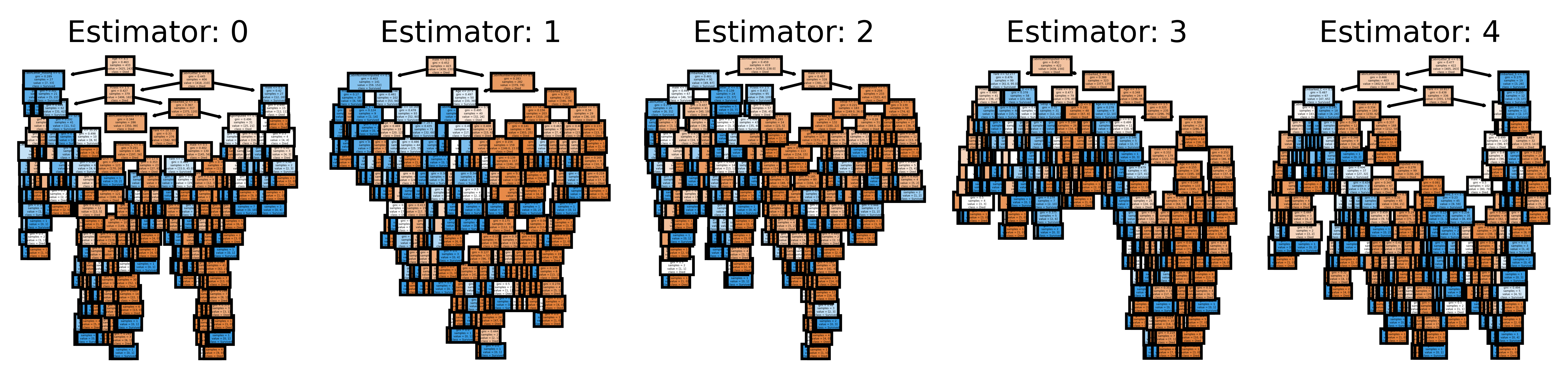

7 Comparing Performance

def train_and_run(model):
    model.fit(X_train,y_train)
    y_pred_train = model.predict(X_train)
    y_pred_test = model.predict(X_test)
    accuracy_train = np.mean(y_pred_train == y_train)
    accuracy_test = np.mean(y_pred_test == y_test)

    print (f'Accuracy of predicting training data = {accuracy_train:.3f}')
    print (f'Accuracy of predicting test data = {accuracy_test:.3f}')

    print(f"F1 score: no averaging = {[f'{i:.3f}' for i in f1_score(y_test, y_pred_test, average=None)]}")
    print(f"F1 score: micro = {f1_score(y_test, y_pred_test, average="micro"):.3f}")
    print(f"F1 score: macro = {f1_score(y_test, y_pred_test, average="macro"):.3f}")
    print(f"F1 score: weighted = {f1_score(y_test, y_pred_test, average="weighted"):.3f}")

from sklearn.tree import DecisionTreeClassifier
train_and_run(model = DecisionTreeClassifier())

Accuracy of predicting training data = 0.984
Accuracy of predicting test data = 0.758
F1 score: no averaging = ['0.795', '0.703']
F1 score: micro = 0.758
F1 score: macro = 0.749
F1 score: weighted = 0.759

np.random.seed(42)
train_and_run(model = RandomForestClassifier(random_state=42))

Accuracy of predicting training data = 0.984
Accuracy of predicting test data = 0.794
F1 score: no averaging = ['0.830', '0.739']
F1 score: micro = 0.794
F1 score: macro = 0.784
F1 score: weighted = 0.793

7.0.0.1 Random Forest

np.random.seed(42)

random_forest_model = RandomForestClassifier(random_state=42)
random_forest_model = random_forest_model.fit(X_train,y_train)

y_pred_train_rf = random_forest_model.predict(X_train)
y_pred_test_rf = random_forest_model.predict(X_test)

roc_curve_rf = RocCurveDisplay.from_estimator(
    random_forest_model, X_test, y_test
)

confusion_matrix_rf = ConfusionMatrixDisplay(
    confusion_matrix=confusion_matrix(
        y_true=y_test,
        y_pred=y_pred_test_rf
        ),
        display_labels=["Died", "Survived"]
)

confusion_matrix_rf_normalised = ConfusionMatrixDisplay(
    confusion_matrix=confusion_matrix(
        y_true=y_test,
        y_pred=y_pred_test_rf,
        normalize='true'
        ),
        display_labels=["Died", "Survived"]
)

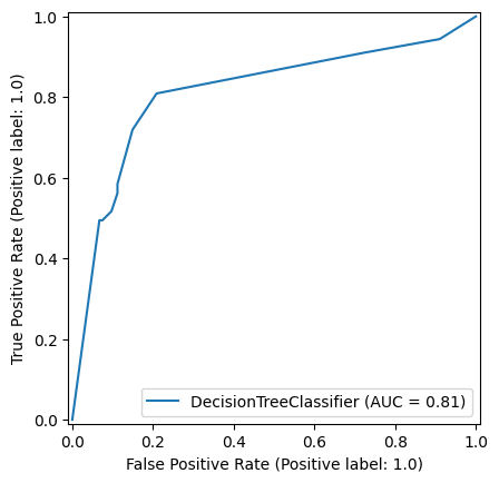
7.0.0.2 Decision Tree

np.random.seed(42)

decision_tree_model = DecisionTreeClassifier(max_depth=6)
decision_tree_model = decision_tree_model.fit(X_train,y_train)

y_pred_train_dt = decision_tree_model.predict(X_train)
y_pred_test_dt = decision_tree_model.predict(X_test)

roc_curve_dt = RocCurveDisplay.from_estimator(
    decision_tree_model, X_test, y_test
)

confusion_matrix_dt = ConfusionMatrixDisplay(
    confusion_matrix=confusion_matrix(
        y_true=y_test,
        y_pred=y_pred_test_dt
        ),
        display_labels=["Died", "Survived"]
)

confusion_matrix_dt_normalised = ConfusionMatrixDisplay(
    confusion_matrix=confusion_matrix(
        y_true=y_test,
        y_pred=y_pred_test_dt,
        normalize='true'
        ),
        display_labels=["Died", "Survived"]
)

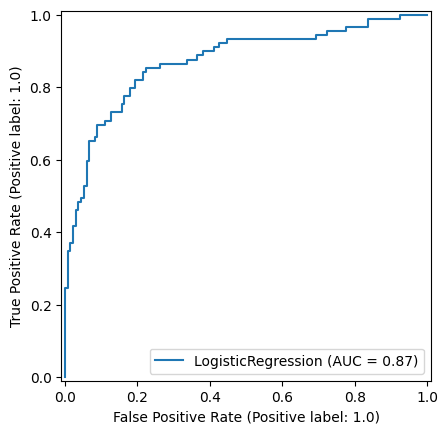
7.0.0.3 Logistic Regression

from sklearn.linear_model import LogisticRegression
from sklearn.preprocessing import StandardScaler

np.random.seed(42)

def standardise_data(X_train, X_test):

    # Initialise a new scaling object for normalising input data
    sc = StandardScaler()

    # Apply the scaler to the training and test sets
    train_std=sc.fit_transform(X_train)
    test_std=sc.fit_transform(X_test)

    return train_std, test_std

X_train_standardised, X_test_standardised = standardise_data(X_train, X_test)

logistic_regression_model = LogisticRegression()
logistic_regression_model.fit(X_train_standardised,y_train)

y_pred_train_lr = logistic_regression_model.predict(X_train_standardised)
y_pred_test_lr = logistic_regression_model.predict(X_test_standardised)

roc_curve_lr = RocCurveDisplay.from_estimator(
    logistic_regression_model, X_test_standardised, y_test
)

confusion_matrix_lr = ConfusionMatrixDisplay(
    confusion_matrix=confusion_matrix(
        y_true=y_test,
        y_pred=y_pred_test_lr
        ),
        display_labels=["Died", "Survived"]
)

confusion_matrix_lr_normalised = ConfusionMatrixDisplay(
    confusion_matrix=confusion_matrix(
        y_true=y_test,
        y_pred=y_pred_test_lr,
        normalize='true'
        ),
        display_labels=["Died", "Survived"]
)

fig, (ax1, ax2, ax3) = plt.subplots(1, 3, figsize=(14, 5))
confusion_matrix_rf.plot(ax=ax1)
ax1.title.set_text('Random Forest')

confusion_matrix_dt.plot(ax=ax2)
ax2.title.set_text('Decision Tree')

confusion_matrix_lr.plot(ax=ax3)
ax3.title.set_text('Logistic Regression')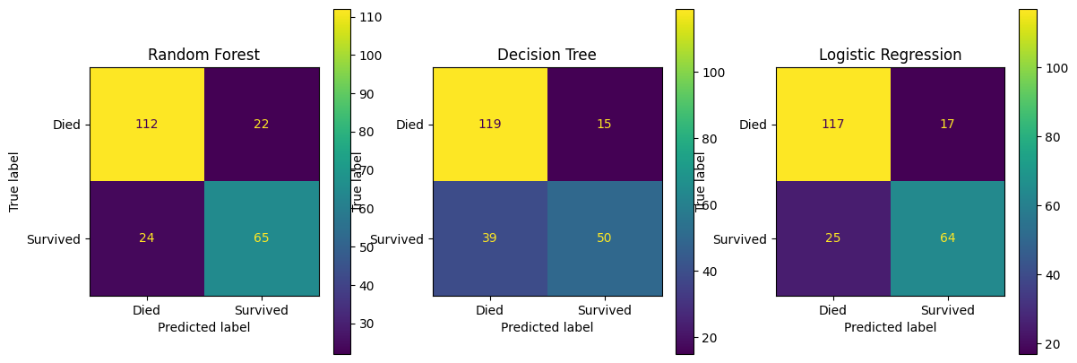

fig, (ax1, ax2, ax3) = plt.subplots(1, 3, figsize=(14, 5))
confusion_matrix_rf_normalised.plot(ax=ax1)
ax1.title.set_text('Random Forest - Normalised')

confusion_matrix_dt_normalised.plot(ax=ax2)
ax2.title.set_text('Decision Tree - Normalised')

confusion_matrix_lr_normalised.plot(ax=ax3)
ax3.title.set_text('Logistic Regression - Normalised')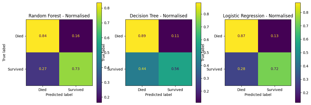

fig, (ax1, ax2, ax3) = plt.subplots(1, 3, figsize=(14, 5))

roc_curve_rf.plot(ax=ax1)
ax1.title.set_text('Random Forest')
ax1.plot([0, 1], [0, 1], color='darkblue', linestyle='--')

roc_curve_dt.plot(ax=ax2)
ax2.title.set_text('Decision Tree')
ax2.plot([0, 1], [0, 1], color='darkblue', linestyle='--')

roc_curve_lr.plot(ax=ax3)
ax3.title.set_text('Logistic Regression')
ax3.plot([0, 1], [0, 1], color='darkblue', linestyle='--')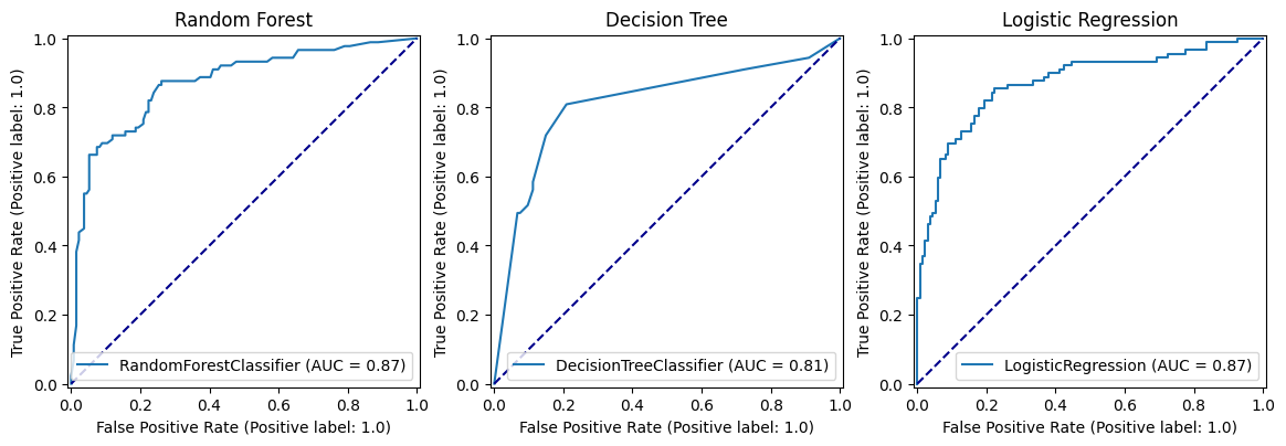

7.1 Hyperparameters

7.1.1 n estimators (trees per forest)

accuracy_results = []

for i in range(10, 500, 10):
    model = model = RandomForestClassifier(n_estimators=i, random_state=42)
    model.fit(X_train,y_train)
    y_pred_train = model.predict(X_train)
    y_pred_test = model.predict(X_test)
    accuracy_train = np.mean(y_pred_train == y_train)
    accuracy_test = np.mean(y_pred_test == y_test)
    accuracy_results.append({'accuracy_train': accuracy_train, 'accuracy_test': accuracy_test, 'n_estimators': i})

px.line(pd.DataFrame(accuracy_results).melt(id_vars='n_estimators'),
        x='n_estimators', y='value', color='variable')

Unable to display output for mime type(s): application/vnd.plotly.v1+json

pd.DataFrame(accuracy_results).set_index("n_estimators").sort_values(by=["accuracy_test"], ascending=False)

	accuracy_train	accuracy_test
n_estimators
30	0.980539	0.807175
40	0.980539	0.807175
50	0.982036	0.802691
20	0.980539	0.802691
10	0.976048	0.798206
60	0.983533	0.798206
70	0.983533	0.798206
80	0.983533	0.798206
90	0.983533	0.798206
120	0.983533	0.793722
100	0.983533	0.793722
110	0.983533	0.793722
210	0.983533	0.793722
450	0.983533	0.789238
440	0.983533	0.789238
260	0.983533	0.789238
240	0.983533	0.789238
230	0.983533	0.789238
220	0.983533	0.789238
250	0.983533	0.789238
200	0.983533	0.789238
180	0.983533	0.789238
170	0.983533	0.789238
160	0.983533	0.789238
150	0.983533	0.789238
190	0.983533	0.789238
130	0.983533	0.789238
140	0.983533	0.789238
420	0.983533	0.784753
400	0.983533	0.784753
410	0.983533	0.784753
460	0.983533	0.784753
430	0.983533	0.784753
380	0.983533	0.784753
470	0.983533	0.784753
480	0.983533	0.784753
390	0.983533	0.784753
350	0.983533	0.784753
370	0.983533	0.784753
360	0.983533	0.784753
340	0.983533	0.784753
330	0.983533	0.784753
320	0.983533	0.784753
310	0.983533	0.784753
300	0.983533	0.784753
290	0.983533	0.784753
280	0.983533	0.784753
270	0.983533	0.784753
490	0.983533	0.784753

7.1.2 n estimators (trees per forest) - with max depth of 8

accuracy_results = []

for i in range(10, 200, 10):
    model = RandomForestClassifier(n_estimators=i, random_state=42, max_depth=8)
    model.fit(X_train,y_train)
    y_pred_train = model.predict(X_train)
    y_pred_test = model.predict(X_test)
    accuracy_train = np.mean(y_pred_train == y_train)
    accuracy_test = np.mean(y_pred_test == y_test)
    accuracy_results.append({'accuracy_train': accuracy_train, 'accuracy_test': accuracy_test, 'n_estimators': i})

px.line(pd.DataFrame(accuracy_results).melt(id_vars='n_estimators'),
        x='n_estimators', y='value', color='variable')

Unable to display output for mime type(s): application/vnd.plotly.v1+json

pd.DataFrame(accuracy_results).set_index("n_estimators").sort_values(by=["accuracy_test"], ascending=False)

	accuracy_train	accuracy_test
n_estimators
190	0.919162	0.829596
180	0.922156	0.829596
170	0.923653	0.829596
150	0.922156	0.829596
140	0.922156	0.829596
90	0.919162	0.829596
110	0.920659	0.825112
160	0.923653	0.825112
130	0.920659	0.825112
10	0.892216	0.825112
80	0.920659	0.825112
70	0.920659	0.825112
50	0.919162	0.825112
100	0.920659	0.825112
120	0.920659	0.820628
20	0.902695	0.816143
40	0.913174	0.816143
60	0.920659	0.811659
30	0.914671	0.811659

np.random.seed(42)

best_n_estimators = pd.DataFrame(accuracy_results).sort_values(by=["accuracy_test"], ascending=False).head(1)['n_estimators'].values[0]

model = RandomForestClassifier(n_estimators=best_n_estimators, random_state=42, max_depth=8)
model.fit(X_train,y_train)
y_pred_train = model.predict(X_train)
y_pred_test = model.predict(X_test)

roc_curve = RocCurveDisplay.from_estimator(
    model, X_test, y_test
)

fig = roc_curve.figure_
ax = roc_curve.ax_


ax.plot([0, 1], [0, 1], color='darkblue', linestyle='--')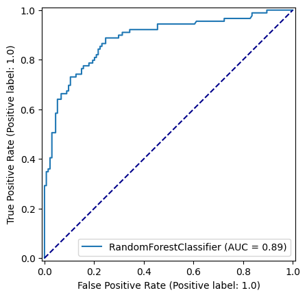

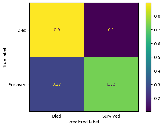
ConfusionMatrixDisplay(
    confusion_matrix=confusion_matrix(
        y_true=y_test,
        y_pred=y_pred_test
        ),
        display_labels=["Died", "Survived"]
).plot()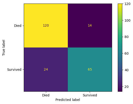

ConfusionMatrixDisplay(
    confusion_matrix=confusion_matrix(
        y_true=y_test,
        y_pred=y_pred_test,
        normalize='true'
        ),
        display_labels=["Died", "Survived"]
).plot()