4  Decision Trees for Classification (Titanic Dataset)

import numpy as np
import pandas as pd
# Import machine learning methods
from sklearn.tree import DecisionTreeClassifier, plot_tree
from sklearn.model_selection import train_test_split
import matplotlib.pyplot as plt
%matplotlib inline
import plotly.express as px
from sklearn.metrics import auc, roc_curve, RocCurveDisplay, f1_score, precision_score, \
                            recall_score, confusion_matrix, ConfusionMatrixDisplay, \
                            classification_report, precision_recall_fscore_support

np.random.seed(42)

download_required = True

if download_required:

    # Download processed data:
    address = 'https://raw.githubusercontent.com/MichaelAllen1966/' + \
                '1804_python_healthcare/master/titanic/data/processed_data.csv'

    data = pd.read_csv(address)

    # Create a data subfolder if one does not already exist
    import os
    data_directory ='../datasets/'
    if not os.path.exists(data_directory):
        os.makedirs(data_directory)

    # Save data
    data.to_csv(data_directory + 'processed_titanic_data.csv', index=False)

data = pd.read_csv('../datasets/processed_titanic_data.csv')
# Make all data 'float' type
data = data.astype(float)

data.head(10)

	PassengerId	Survived	Pclass	Age	SibSp	Parch	Fare	AgeImputed	EmbarkedImputed	CabinLetterImputed	...	Embarked_missing	CabinLetter_A	CabinLetter_B	CabinLetter_C	CabinLetter_D	CabinLetter_E	CabinLetter_F	CabinLetter_G	CabinLetter_T	CabinLetter_missing
0	1.0	0.0	3.0	22.0	1.0	0.0	7.2500	0.0	0.0	1.0	...	0.0	0.0	0.0	0.0	0.0	0.0	0.0	0.0	0.0	1.0
1	2.0	1.0	1.0	38.0	1.0	0.0	71.2833	0.0	0.0	0.0	...	0.0	0.0	0.0	1.0	0.0	0.0	0.0	0.0	0.0	0.0
2	3.0	1.0	3.0	26.0	0.0	0.0	7.9250	0.0	0.0	1.0	...	0.0	0.0	0.0	0.0	0.0	0.0	0.0	0.0	0.0	1.0
3	4.0	1.0	1.0	35.0	1.0	0.0	53.1000	0.0	0.0	0.0	...	0.0	0.0	0.0	1.0	0.0	0.0	0.0	0.0	0.0	0.0
4	5.0	0.0	3.0	35.0	0.0	0.0	8.0500	0.0	0.0	1.0	...	0.0	0.0	0.0	0.0	0.0	0.0	0.0	0.0	0.0	1.0
5	6.0	0.0	3.0	28.0	0.0	0.0	8.4583	1.0	0.0	1.0	...	0.0	0.0	0.0	0.0	0.0	0.0	0.0	0.0	0.0	1.0
6	7.0	0.0	1.0	54.0	0.0	0.0	51.8625	0.0	0.0	0.0	...	0.0	0.0	0.0	0.0	0.0	1.0	0.0	0.0	0.0	0.0
7	8.0	0.0	3.0	2.0	3.0	1.0	21.0750	0.0	0.0	1.0	...	0.0	0.0	0.0	0.0	0.0	0.0	0.0	0.0	0.0	1.0
8	9.0	1.0	3.0	27.0	0.0	2.0	11.1333	0.0	0.0	1.0	...	0.0	0.0	0.0	0.0	0.0	0.0	0.0	0.0	0.0	1.0
9	10.0	1.0	2.0	14.0	1.0	0.0	30.0708	0.0	0.0	1.0	...	0.0	0.0	0.0	0.0	0.0	0.0	0.0	0.0	0.0	1.0

10 rows × 26 columns

data.describe()

	PassengerId	Survived	Pclass	Age	SibSp	Parch	Fare	AgeImputed	EmbarkedImputed	CabinLetterImputed	...	Embarked_missing	CabinLetter_A	CabinLetter_B	CabinLetter_C	CabinLetter_D	CabinLetter_E	CabinLetter_F	CabinLetter_G	CabinLetter_T	CabinLetter_missing
count	891.000000	891.000000	891.000000	891.000000	891.000000	891.000000	891.000000	891.000000	891.000000	891.000000	...	891.000000	891.000000	891.000000	891.000000	891.000000	891.000000	891.000000	891.000000	891.000000	891.000000
mean	446.000000	0.383838	2.308642	29.361582	0.523008	0.381594	32.204208	0.198653	0.002245	0.771044	...	0.002245	0.016835	0.052750	0.066218	0.037037	0.035915	0.014590	0.004489	0.001122	0.771044
std	257.353842	0.486592	0.836071	13.019697	1.102743	0.806057	49.693429	0.399210	0.047351	0.420397	...	0.047351	0.128725	0.223659	0.248802	0.188959	0.186182	0.119973	0.066890	0.033501	0.420397
min	1.000000	0.000000	1.000000	0.420000	0.000000	0.000000	0.000000	0.000000	0.000000	0.000000	...	0.000000	0.000000	0.000000	0.000000	0.000000	0.000000	0.000000	0.000000	0.000000	0.000000
25%	223.500000	0.000000	2.000000	22.000000	0.000000	0.000000	7.910400	0.000000	0.000000	1.000000	...	0.000000	0.000000	0.000000	0.000000	0.000000	0.000000	0.000000	0.000000	0.000000	1.000000
50%	446.000000	0.000000	3.000000	28.000000	0.000000	0.000000	14.454200	0.000000	0.000000	1.000000	...	0.000000	0.000000	0.000000	0.000000	0.000000	0.000000	0.000000	0.000000	0.000000	1.000000
75%	668.500000	1.000000	3.000000	35.000000	1.000000	0.000000	31.000000	0.000000	0.000000	1.000000	...	0.000000	0.000000	0.000000	0.000000	0.000000	0.000000	0.000000	0.000000	0.000000	1.000000
max	891.000000	1.000000	3.000000	80.000000	8.000000	6.000000	512.329200	1.000000	1.000000	1.000000	...	1.000000	1.000000	1.000000	1.000000	1.000000	1.000000	1.000000	1.000000	1.000000	1.000000

8 rows × 26 columns

# Drop Passengerid (axis=1 indicates we are removing a column rather than a row)
# We drop passenger ID as it is not original data
# inplace=True means change the dataframe itself - don't create a copy with this column dropped

data.drop('PassengerId', inplace=True, axis=1)

4.1 Divide into X (features) and y (labels)

X = data.drop('Survived',axis=1) # X = all 'data' except the 'survived' column
y = data['Survived'] # y = 'survived' column from 'data'

4.2 Divide into training and tets sets

X_train, X_test, y_train, y_test = train_test_split(X, y, test_size = 0.25)

4.3 Fit decision tree model

model = DecisionTreeClassifier() # Create a Decision Tree Model
model = model.fit(X_train,y_train) # Fit the model using our training data

4.4 Predict values

# Predict training and test set labels
y_pred_train = model.predict(X_train)
y_pred_test = model.predict(X_test)

4.5 Calculate accuracy

# The shorthand below says to check each predicted y value against the actual
# y value in the training data.  This gives a list of True and False values
# for each prediction, where True indicates the predicted value matches the
# actual value.  Then we take the mean of these Boolean values, which gives
# us a proportion (where if all values were True, the proportion would be 1.0)
# If you want to see why that works, just uncomment the following line of code
# to see what y_pred_train == y_train is doing.
# print (y_pred_train == y_train)
accuracy_train = np.mean(y_pred_train == y_train)
accuracy_test = np.mean(y_pred_test == y_test)

print (f'Accuracy of predicting training data = {accuracy_train:3f}')
print (f'Accuracy of predicting test data = {accuracy_test:3f}')

Accuracy of predicting training data = 0.983533
Accuracy of predicting test data = 0.766816

# Show first ten predicted classes
classes = model.predict(X_test)
classes[0:10]

array([0., 1., 0., 1., 1., 1., 1., 0., 0., 1.])

# Show first ten predicted probabilities
probabilities = model.predict_proba(X_test)
probabilities[0:10]

array([[1.        , 0.        ],
       [0.        , 1.        ],
       [1.        , 0.        ],
       [0.        , 1.        ],
       [0.        , 1.        ],
       [0.        , 1.        ],
       [0.16666667, 0.83333333],
       [1.        , 0.        ],
       [1.        , 0.        ],
       [0.        , 1.        ]])

4.6 Plot tree

fig = plot_tree(model)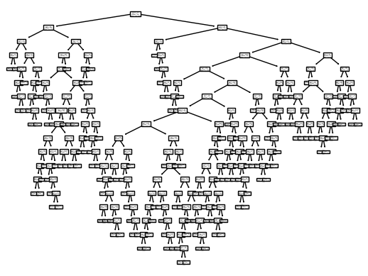

fig = plot_tree(
    model,
    feature_names=data.drop('Survived',axis=1).columns.tolist(),
    class_names=['Died', 'Survived'],
    filled=True
    )

4.7 Following Nodes

https://scikit-learn.org/stable/auto_examples/tree/plot_unveil_tree_structure.html#sphx-glr-auto-examples-tree-plot-unveil-tree-structure-py

5 Tweaking DT Parameters

def train_and_run_dt(model):
    model.fit(X_train,y_train)
    y_pred_train = model.predict(X_train)
    y_pred_test = model.predict(X_test)
    accuracy_train = np.mean(y_pred_train == y_train)
    accuracy_test = np.mean(y_pred_test == y_test)

    print (f'Accuracy of predicting training data = {accuracy_train:.3f}')
    print (f'Accuracy of predicting test data = {accuracy_test:.3f}')

    print (f'Precision on test data = {precision_score(y_test, y_pred_test, average='micro'):.3f}')
    print (f'Recall on test data = {recall_score(y_test, y_pred_test, average='micro'):.3f}')
    print (f'Specificity on test data = {precision_score(y_test, y_pred_test, average='micro', pos_label=0):.3f}')

recall_score(y_test, y_pred_test, average='micro')

0.7668161434977578

precision_score(y_test, y_pred_test, pos_label=0)

0.8106060606060606

train_and_run_dt(model = DecisionTreeClassifier())

Accuracy of predicting training data = 0.984
Accuracy of predicting test data = 0.758
Precision on test data = 0.758
Recall on test data = 0.758
Specificity on test data = 0.758

c:\HSMA\_HSMA 6\Sammi's Sessions\h6_4d_decision_trees_random_forests\h6_4d_decision_trees_random_forests\.venv\Lib\site-packages\sklearn\metrics\_classification.py:1561: UserWarning:

Note that pos_label (set to 0) is ignored when average != 'binary' (got 'micro'). You may use labels=[pos_label] to specify a single positive class.

5.0.1 Min Samples Leaf

train_and_run_dt(model = DecisionTreeClassifier(min_samples_leaf=5))

Accuracy of predicting training data = 0.883
Accuracy of predicting test data = 0.830
Precision on test data = 0.830
Recall on test data = 0.830
Specificity on test data = 0.830

c:\HSMA\_HSMA 6\Sammi's Sessions\h6_4d_decision_trees_random_forests\h6_4d_decision_trees_random_forests\.venv\Lib\site-packages\sklearn\metrics\_classification.py:1561: UserWarning:

Note that pos_label (set to 0) is ignored when average != 'binary' (got 'micro'). You may use labels=[pos_label] to specify a single positive class.

accuracy_results = []

for i in range(1, 15, 1):
    model = DecisionTreeClassifier(min_samples_leaf=i, random_state=42)
    model.fit(X_train,y_train)
    y_pred_train = model.predict(X_train)
    y_pred_test = model.predict(X_test)
    accuracy_train = np.mean(y_pred_train == y_train)
    accuracy_test = np.mean(y_pred_test == y_test)
    accuracy_results.append({'accuracy_train': accuracy_train, 'accuracy_test': accuracy_test, 'min_samples_leaf': i})

px.line(pd.DataFrame(accuracy_results).melt(id_vars='min_samples_leaf'),
        x='min_samples_leaf', y='value', color='variable')

Unable to display output for mime type(s): application/vnd.plotly.v1+json

5.0.1.1 Min Samples Split

train_and_run_dt(model = DecisionTreeClassifier(min_samples_split=5))

Accuracy of predicting training data = 0.945
Accuracy of predicting test data = 0.767
Precision on test data = 0.767
Recall on test data = 0.767
Specificity on test data = 0.767

c:\HSMA\_HSMA 6\Sammi's Sessions\h6_4d_decision_trees_random_forests\h6_4d_decision_trees_random_forests\.venv\Lib\site-packages\sklearn\metrics\_classification.py:1561: UserWarning:

Note that pos_label (set to 0) is ignored when average != 'binary' (got 'micro'). You may use labels=[pos_label] to specify a single positive class.

accuracy_results = []

for i in range(2, 15, 1):
    model = DecisionTreeClassifier(min_samples_split=i)
    model.fit(X_train,y_train)
    y_pred_train = model.predict(X_train)
    y_pred_test = model.predict(X_test)
    accuracy_train = np.mean(y_pred_train == y_train)
    accuracy_test = np.mean(y_pred_test == y_test)
    accuracy_results.append({'accuracy_train': accuracy_train, 'accuracy_test': accuracy_test, 'min_samples_split': i})

px.line(pd.DataFrame(accuracy_results).melt(id_vars='min_samples_split'),
        x='min_samples_split', y='value', color='variable')

Unable to display output for mime type(s): application/vnd.plotly.v1+json

train_and_run_dt(model = DecisionTreeClassifier())

Accuracy of predicting training data = 0.984
Accuracy of predicting test data = 0.744
Precision on test data = 0.744
Recall on test data = 0.744
Specificity on test data = 0.744

c:\HSMA\_HSMA 6\Sammi's Sessions\h6_4d_decision_trees_random_forests\h6_4d_decision_trees_random_forests\.venv\Lib\site-packages\sklearn\metrics\_classification.py:1561: UserWarning:

Note that pos_label (set to 0) is ignored when average != 'binary' (got 'micro'). You may use labels=[pos_label] to specify a single positive class.

train_and_run_dt(model = DecisionTreeClassifier(max_depth=5))

Accuracy of predicting training data = 0.861
Accuracy of predicting test data = 0.807
Precision on test data = 0.807
Recall on test data = 0.807
Specificity on test data = 0.807

c:\HSMA\_HSMA 6\Sammi's Sessions\h6_4d_decision_trees_random_forests\h6_4d_decision_trees_random_forests\.venv\Lib\site-packages\sklearn\metrics\_classification.py:1561: UserWarning:

Note that pos_label (set to 0) is ignored when average != 'binary' (got 'micro'). You may use labels=[pos_label] to specify a single positive class.

train_and_run_dt(model = DecisionTreeClassifier(max_depth=3))

Accuracy of predicting training data = 0.832
Accuracy of predicting test data = 0.803
Precision on test data = 0.803
Recall on test data = 0.803
Specificity on test data = 0.803

c:\HSMA\_HSMA 6\Sammi's Sessions\h6_4d_decision_trees_random_forests\h6_4d_decision_trees_random_forests\.venv\Lib\site-packages\sklearn\metrics\_classification.py:1561: UserWarning:

Note that pos_label (set to 0) is ignored when average != 'binary' (got 'micro'). You may use labels=[pos_label] to specify a single positive class.

train_and_run_dt(model = DecisionTreeClassifier(max_depth=7))

Accuracy of predicting training data = 0.891
Accuracy of predicting test data = 0.789
Precision on test data = 0.789
Recall on test data = 0.789
Specificity on test data = 0.789

c:\HSMA\_HSMA 6\Sammi's Sessions\h6_4d_decision_trees_random_forests\h6_4d_decision_trees_random_forests\.venv\Lib\site-packages\sklearn\metrics\_classification.py:1561: UserWarning:

Note that pos_label (set to 0) is ignored when average != 'binary' (got 'micro'). You may use labels=[pos_label] to specify a single positive class.

accuracy_results = []

for i in range(1, 15, 1):
    model = model = DecisionTreeClassifier(max_depth=i)
    model.fit(X_train,y_train)
    y_pred_train = model.predict(X_train)
    y_pred_test = model.predict(X_test)
    accuracy_train = np.mean(y_pred_train == y_train)
    accuracy_test = np.mean(y_pred_test == y_test)
    accuracy_results.append({'accuracy_train': accuracy_train, 'accuracy_test': accuracy_test, 'max_depth': i})

px.line(pd.DataFrame(accuracy_results).melt(id_vars='max_depth'),
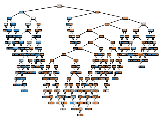
        x='max_depth', y='value', color='variable')

Unable to display output for mime type(s): application/vnd.plotly.v1+json

fig, ax = plt.subplots(figsize=(10,8))

model = DecisionTreeClassifier()
model = model.fit(X_train, y_train)
tree_plot = plot_tree(model,
    feature_names=data.drop('Survived',axis=1).columns.tolist(),
    class_names=['Died', 'Survived'],
    filled=True,
    ax=ax
    )

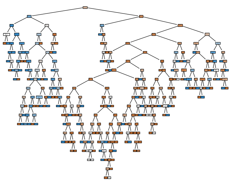
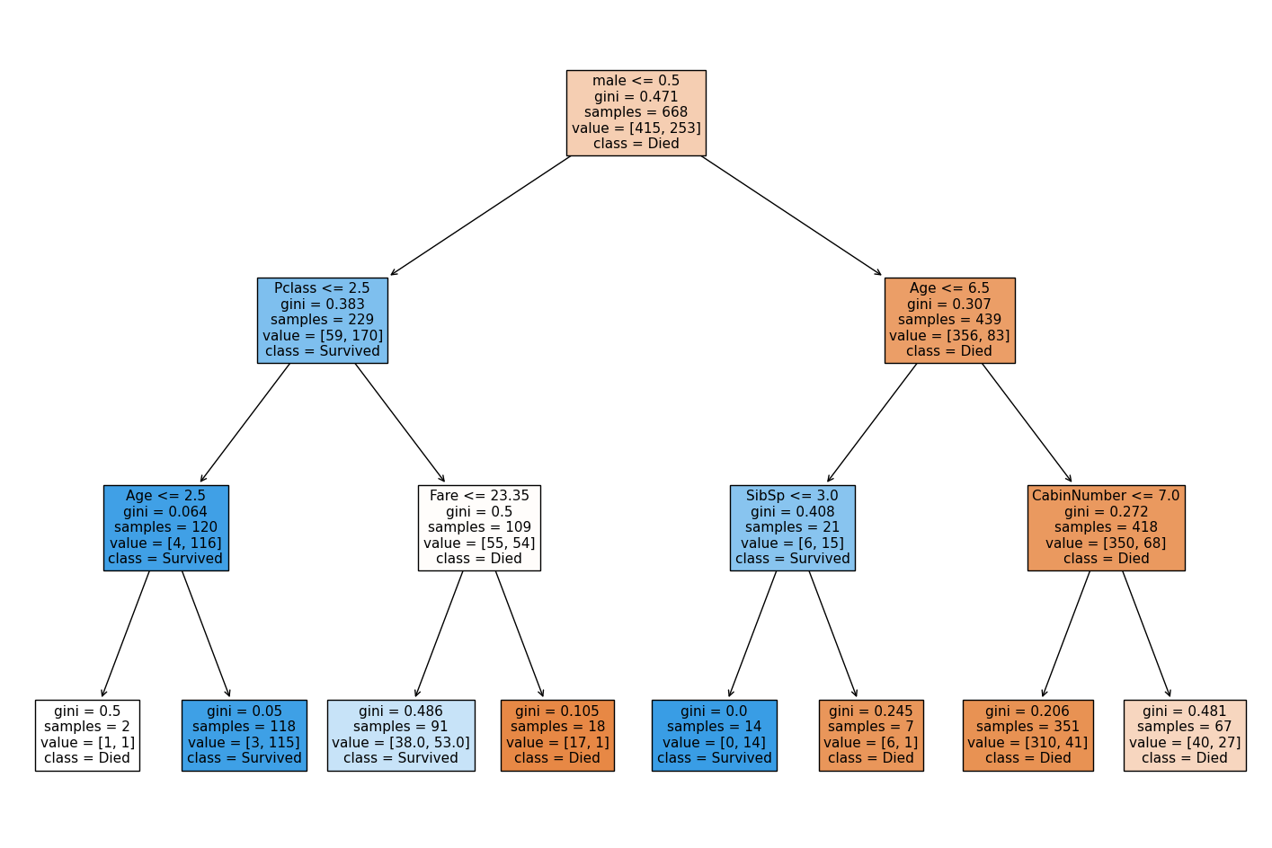
fig, ax = plt.subplots(figsize=(18,12))

model = DecisionTreeClassifier(max_depth=3)
model = model.fit(X_train, y_train)
tree_plot = plot_tree(model,
    feature_names=data.drop('Survived',axis=1).columns.tolist(),
    class_names=['Died', 'Survived'],
    filled=True,
    ax=ax,
    fontsize=11
    )

6 Compare with our log reg

from sklearn.linear_model import LogisticRegression
from sklearn.model_selection import train_test_split
from sklearn.preprocessing import StandardScaler

def standardise_data(X_train, X_test):

    # Initialise a new scaling object for normalising input data
    sc = StandardScaler()

    # Apply the scaler to the training and test sets
    train_std=sc.fit_transform(X_train)
    test_std=sc.fit_transform(X_test)

    return train_std, test_std

X_train_standardised, X_test_standardised = standardise_data(X_train, X_test)

model = LogisticRegression()
model.fit(X_train_standardised,y_train)

LogisticRegression()

In a Jupyter environment, please rerun this cell to show the HTML representation or trust the notebook.
On GitHub, the HTML representation is unable to render, please try loading this page with nbviewer.org.

# Predict training and test set labels
y_pred_train = model.predict(X_train_standardised)
y_pred_test = model.predict(X_test_standardised)

# The shorthand below says to check each predicted y value against the actual
# y value in the training data.  This gives a list of True and False values
# for each prediction, where True indicates the predicted value matches the
# actual value.  Then we take the mean of these Boolean values, which gives
# us a proportion (where if all values were True, the proportion would be 1.0)
# If you want to see why that works, just uncomment the following line of code
# to see what y_pred_train == y_train is doing.
# print (y_pred_train == y_train)
accuracy_train = np.mean(y_pred_train == y_train)
accuracy_test = np.mean(y_pred_test == y_test)

print (f'Accuracy of predicting training data = {accuracy_train}')
print (f'Accuracy of predicting test data = {accuracy_test}')

Accuracy of predicting training data = 0.8083832335329342
Accuracy of predicting test data = 0.8116591928251121

Best train accuracy seen in DT: 0.823 Train accuracy seen in LR: 0.805

Best test accuracy seen in DT: 0.820 Test accuracy seen in LR: 0.798

6.1 Post pruning

https://ranvir.xyz/blog/practical-approach-to-tree-pruning-using-sklearn/

https://scikit-learn.org/stable/auto_examples/tree/plot_cost_complexity_pruning.html

import matplotlib.pyplot as plt

model = DecisionTreeClassifier()
path = model.cost_complexity_pruning_path(X_train, y_train)

ccp_alphas, impurities = path.ccp_alphas, path.impurities

plt.figure(figsize=(10, 6))
plt.plot(ccp_alphas, impurities)
plt.xlabel("effective alpha")
plt.ylabel("total impurity of leaves")

Text(0, 0.5, 'total impurity of leaves')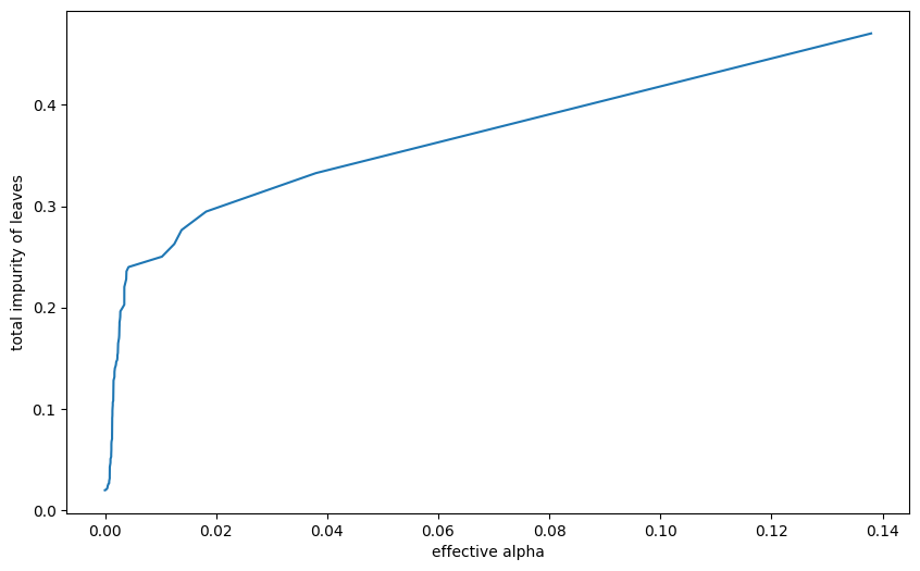

models = []

for ccp_alpha in ccp_alphas:
    model = DecisionTreeClassifier(random_state=0, ccp_alpha=ccp_alpha)
    model.fit(X_train, y_train)
    models.append(model)

tree_depths = [model.tree_.max_depth for model in models]
plt.figure(figsize=(10,  6))
plt.plot(ccp_alphas[:-1], tree_depths[:-1])
plt.xlabel("effective alpha")
plt.ylabel("total depth")

Text(0, 0.5, 'total depth')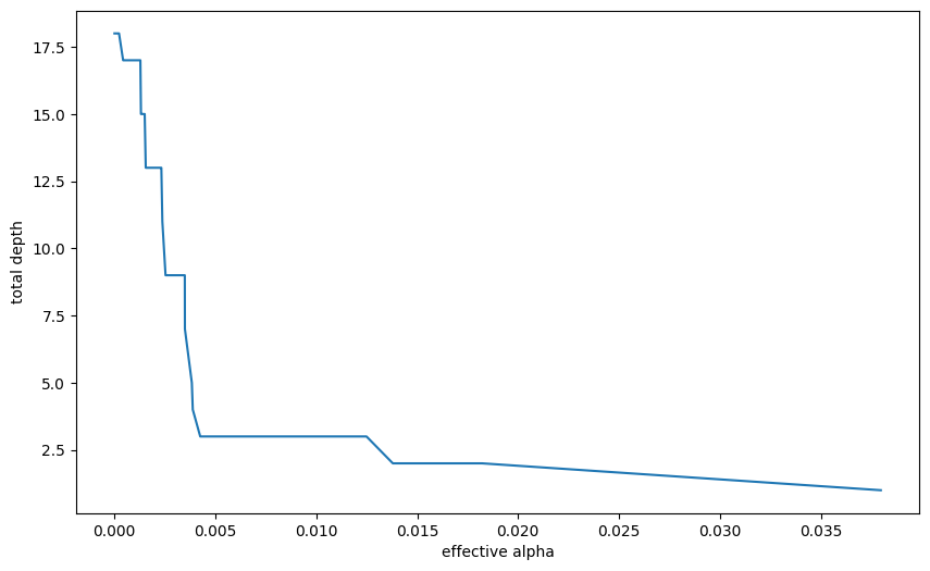

from sklearn.metrics import accuracy_score

acc_scores = [accuracy_score(y_test, model.predict(X_test)) for model in models]

tree_depths = [model.tree_.max_depth for model in models]
plt.figure(figsize=(10,  6))
plt.grid()
plt.plot(ccp_alphas[:-1], acc_scores[:-1])
plt.xlabel("effective alpha")
plt.ylabel("Accuracy scores")

Text(0, 0.5, 'Accuracy scores')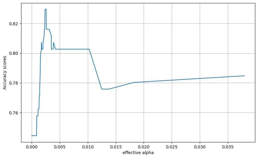

Final model from this approach

train_and_run_dt(DecisionTreeClassifier(random_state=0, ccp_alpha=0.0045))

Accuracy of predicting training data = 0.832
Accuracy of predicting test data = 0.803
Precision on test data = 0.803
Recall on test data = 0.803
Specificity on test data = 0.803

c:\HSMA\_HSMA 6\Sammi's Sessions\h6_4d_decision_trees_random_forests\h6_4d_decision_trees_random_forests\.venv\Lib\site-packages\sklearn\metrics\_classification.py:1561: UserWarning:

Note that pos_label (set to 0) is ignored when average != 'binary' (got 'micro'). You may use labels=[pos_label] to specify a single positive class.

6.2 Exploring metrics in our lr and dt

6.2.1 Decision Tree

decision_tree_model = model = DecisionTreeClassifier(max_depth=6)
decision_tree_model = decision_tree_model.fit(X_train,y_train)
y_pred_train_dt = decision_tree_model.predict(X_train)
y_pred_test_dt = decision_tree_model.predict(X_test)

roc_curve = RocCurveDisplay.from_estimator(
    decision_tree_model, X_test, y_test
)

fig = roc_curve.figure_
ax = roc_curve.ax_


ax.plot([0, 1], [0, 1], color='darkblue', linestyle='--')

np.random.seed(42)

decision_tree_model = DecisionTreeClassifier(max_depth=6)
decision_tree_model = decision_tree_model.fit(X_train,y_train)

y_pred_train_dt = decision_tree_model.predict(X_train)
y_pred_test_dt = decision_tree_model.predict(X_test)

roc_curve_dt = RocCurveDisplay.from_estimator(
    decision_tree_model, X_test, y_test
)

fig = roc_curve_dt.figure_
ax = roc_curve_dt.ax_

ax.plot([0, 1], [0, 1], color='darkblue', linestyle='--')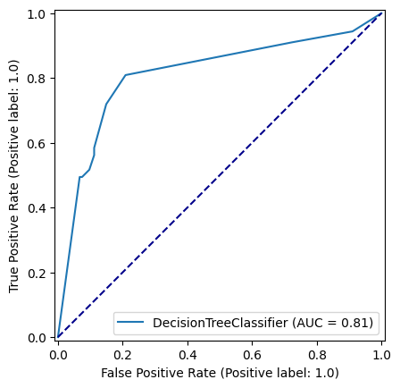

confusion_matrix_dt = ConfusionMatrixDisplay(
    confusion_matrix=confusion_matrix(
        y_true=y_test,
        y_pred=y_pred_test_dt
        ),
        display_labels=["Died", "Survived"]
)

confusion_matrix_dt.plot()

plt.show()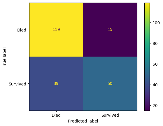

confusion_matrix_dt_normalised = ConfusionMatrixDisplay(
    confusion_matrix=confusion_matrix(
        y_true=y_test,
        y_pred=y_pred_test_dt,
        normalize='true'
        ),
        display_labels=["Died", "Survived"]
)

confusion_matrix_dt_normalised.plot()

plt.show()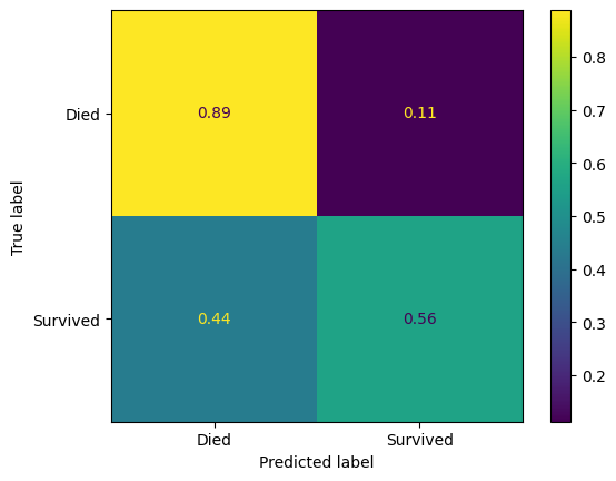

pd.DataFrame(precision_recall_fscore_support(
        y_true=y_test,
        y_pred=y_pred_test_dt,
        average="binary"
        ))

	0
0	0.769231
1	0.561798
2	0.649351
3	NaN

6.2.2 Logistic Regression

from sklearn.linear_model import LogisticRegression
from sklearn.preprocessing import StandardScaler

def standardise_data(X_train, X_test):

    # Initialise a new scaling object for normalising input data
    sc = StandardScaler()

    # Apply the scaler to the training and test sets
    train_std=sc.fit_transform(X_train)
    test_std=sc.fit_transform(X_test)

    return train_std, test_std

X_train_standardised, X_test_standardised = standardise_data(X_train, X_test)

logistic_regression_model = LogisticRegression()
logistic_regression_model = logistic_regression_model.fit(X_train_standardised,y_train)

y_pred_train_lr = logistic_regression_model.predict(X_train_standardised)
y_pred_test_lr = logistic_regression_model.predict(X_test_standardised)

accuracy_train = np.mean(y_pred_train_lr == y_train)
accuracy_test = np.mean(y_pred_test_lr == y_test)

print (f'Accuracy of predicting training data = {accuracy_train}')
print (f'Accuracy of predicting test data = {accuracy_test}')

Accuracy of predicting training data = 0.8083832335329342
Accuracy of predicting test data = 0.8116591928251121

roc_curve_lr = RocCurveDisplay.from_estimator(
    logistic_regression_model, X_test_standardised, y_test
)

fig = roc_curve_lr.figure_
ax = roc_curve_lr.ax_

ax.plot([0, 1], [0, 1], color='darkblue', linestyle='--')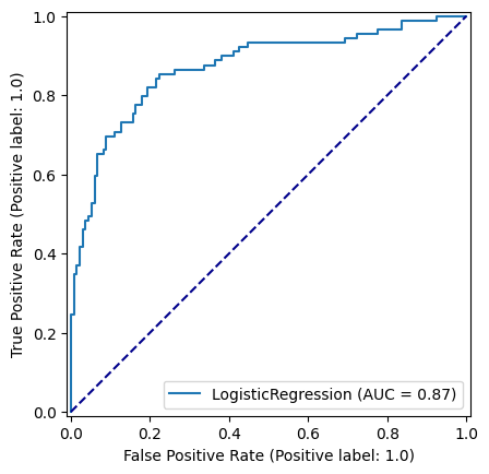

confusion_matrix_lr = ConfusionMatrixDisplay(
    confusion_matrix=confusion_matrix(
        y_true=y_test,
        y_pred=y_pred_test_lr,
        ),
        display_labels=["Died", "Survived"]
)

confusion_matrix_lr.plot()

plt.show()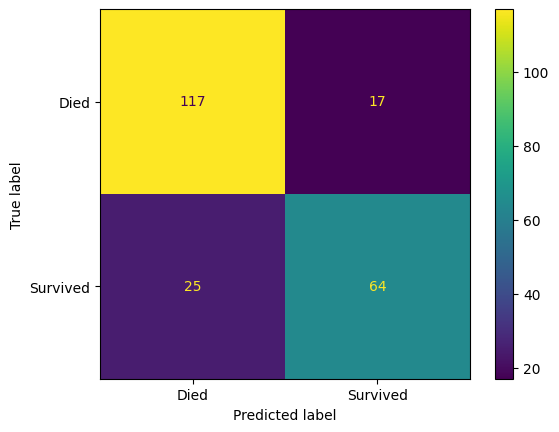

confusion_matrix_lr_normalised = ConfusionMatrixDisplay(
    confusion_matrix=confusion_matrix(
        y_true=y_test,
        y_pred=y_pred_test_lr,
        normalize='true',
        ),
        display_labels=["Died", "Survived"]
)

confusion_matrix_lr_normalised.plot()

plt.show()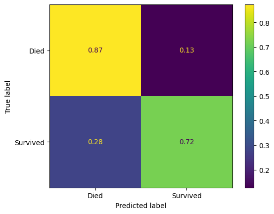

pd.DataFrame(classification_report(
        y_true=y_test,
        y_pred=y_pred_test_lr,
        target_names=["Died", "Survived"],
        output_dict=True
))

	Died	Survived	accuracy	macro avg	weighted avg
precision	0.823944	0.790123	0.811659	0.807034	0.810446
recall	0.873134	0.719101	0.811659	0.796118	0.811659
f1-score	0.847826	0.752941	0.811659	0.800384	0.809957
support	134.000000	89.000000	0.811659	223.000000	223.000000

precision, recall, fbeta, support = precision_recall_fscore_support(
        y_true=y_test,
        y_pred=y_pred_test_lr,
        average="binary"
        )

6.3 Compare confusion matrices

fig, (ax1, ax2) = plt.subplots(1, 2, figsize=(14, 5))
confusion_matrix_dt.plot(ax=ax1)
ax1.title.set_text('Decision Tree')

confusion_matrix_lr.plot(ax=ax2)
ax2.title.set_text('Logistic Regression')

fig, (ax1, ax2) = plt.subplots(1, 2, figsize=(14, 5))
confusion_matrix_dt_normalised.plot(ax=ax1)
ax1.title.set_text('Decision Tree - Normalised')

confusion_matrix_lr_normalised.plot(ax=ax2)
ax2.title.set_text('Logistic Regression - Normalised')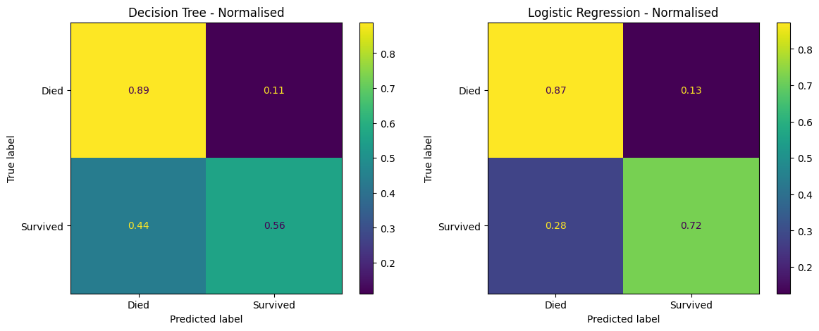

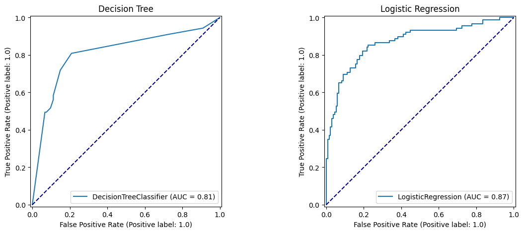
7 Compare ROC Curves

fig, (ax1, ax2) = plt.subplots(1, 2, figsize=(14, 5))
roc_curve_dt.plot(ax=ax1)
ax1.title.set_text('Decision Tree')
ax1.plot([0, 1], [0, 1], color='darkblue', linestyle='--')

roc_curve_lr.plot(ax=ax2)
ax2.title.set_text('Logistic Regression')
ax2.plot([0, 1], [0, 1], color='darkblue', linestyle='--')